Topics

Estimating runtime of algorithm
The notion of time-complexity
Big O Notation and its use in finding time-complexity of an algorithm
Analyze algorithms using Big O notation

Learning Outcomes

By the end of this lesson, you should be able to

Define the time-complexity of an algorithm
Explain how runtime of an algorithm is estimated theoretically
Estimate runtime of a given algorithm or code
Explain the worst case, average case and best case scenarios in analyzing algorithms
Compare the efficiency of different algorithms

Introduction

An algorithm is a sequence of steps to solve a problem. There can be many correct algorithms in that they do what they are supposed to do, but not all algorithms are equally efficient. Usually the most efficient algorithm is used to solve the problem.

Efficiency means how much resources such as time or space is needed by the algorithm. An algorithm that takes a year to solve a problem is not efficient if compared against an algorithm that can solve the same problem in seconds. Likewise, an algorithm that requires a larger portion of computer main memory than another algorithm is not efficient, either. Analyzing algorithms means finding out the efficiency of the algorithms. Doing so allows us to compare different algorithms. The resources used by a program include: CPU time, memory, disk, and network usage. In this lesson we focus on CPU time taken by an algorithm.

In this lesson, we discuss how to estimate the time taken by an algorithm. We introduce a theoretical technique called asymptotic analysis. This tool allows us to compare different algorithms and choose the most efficient one in term of the time it takes to run the algorithm.

Asymptotic Analysis

Motivation

To measure runtime of an algorithm, we can implement it in a programming language, run it on a computer and measure the raw execution time of the algorithms for a specific input. However, there are several limitations with this approach:

this execution time depends on the hardware, the programming language, the compiler, and the input provided.
the same algorithm runs faster on a faster CPU.
the same algorithm takes different running time against different input sizes.
It is not possible to run the algorithm against all possible inputs.

To overcome the above-mentioned limitations, we use a theoretical method called asymptotic analysis to estimate the runtime of an algorithm. The running time obtained using this technique is referred to as time-complexity of the algorithm. Before going further let's see what affects the runtime of an algorithm.

Factors affecting the runtime of an algorithm

The runtime of an algorithm depends mostly on two factors discussed:

The runtime of an algorithm depends on the number of constant time operations performed. Note that it does not depend on the time (e.g., nanoseconds) it takes to perform the operations. A constant time operation is an operation that, for a given processor, always operates in the same amount of time, regardless of input values. Example of constant-time operations are:
- Addition, subtraction, multiplication, and division of fixed-size integer or floating point numbers.
- Assignment of a variable to a fixed-size data value
- Comparison of two fixed-size data values (e.g., x == 0)
- One read/write from/to disk.

The running time of an algorithm depends on both the input size (e.g., the value of a parameter or a field used in the execution of a method) and the work performed on that input.

Consider an extremely simple function that takes a Python list as a parameter, and without examining the list contents, prints the message Array Received . Although the list parameter may vary in size, the amount of work done on the parameter never varies. Thus this algorithm takes the same amount of time no matter how large the list is.

Now consider a function that takes a Python list as a parameter and searches it for a particular value (a linear search). If the size of the list is 10, we have only ten potential positions to look at. But if the size of the list is 1,000,000, then we have one million potential positions to look at. The execution time is directly proportional to the parameter passed to the function, i,e., the list size. Therefore, the running time not only depends on list size but also depends on the operations that the algorithm performs.

Runtime of an algorithm: Average Case, Worst Case, Best Case Analysis

Considering the factors that affect running time of an algorithm, an algorithm's runtime is expressed as a function, T(n), that represents the number of constant time operations performed by the algorithm on an input of size n. If there is more than one input, the functions may have more than one argument.
Because an algorithm's runtime may vary significantly based on the input data, when calculating the number of constant-time operations, T(n), there are three scenarios to consider:

The worst case: T_worst(n) : This case represents the maximum number of operations that might be performed for a given problem size. For example, as discussed above, the linear_search function has to walk through the list to find the given element. In the worst case, it needs to check all of the elements in the list. Therefore, in the worst case, the runtime is proportional to the number of elements in the list and T(N) is a linear function.
The average case, T_avg(n) : The average number of operations that might be performed. In the example of linear_search function, the average number of elements to be checked is n/2. In this case, also T(n) is a linear function.
The best case, T_best(n) : This case represents the scenario where the minimum number of operations are performed by the algorithm. For example, in the linear_search method, the minimum number happens when the elements to be searched is at the beginning of the array. It takes just one operation in the best case (i.e., one check in the list) and T(n) is a constant function.

Clearly, T_best(n) ≤ T_avg(n) ≤ T_worst(n).

We are usually interested in the worst case and T(n) denotes T_worst(n) unless otherwise specified. The reasons are:

The worst-case scenario provides an upper bound for the runtime function, since it covers all inputs, including particularly bad inputs (inputs that leads to large number of operations), that are not covered by an average-case analysis.
The average-case analysis is usually much more difficult to compute. In some instances, the definition of "average" can affect the result.

Finding the growth rate of runtime function

The first step in asymptotic analysis is to find the number of constant time operations performed by the algorithm as a function of input size, e.g., T(n). The next step is to see how the number of operations relate to the input size. That means, we are not interested in the exact number of operations performed. Instead we are interested to see what happens as the size of the problem being solved gets larger. When the input size is doubled, the running time of an algorithm might double, quadruple, or become 1000 times faster depending on the algorithm. For constant-time methods like a method that just prints "Array retrieved", doubling the problem size does not affect the number of operations.

In other words, in asymptotic analysis, we look at the growth rate of the runtime function as the input size grows. That is, how does the execution time increase as the size of the input grows. Some programs take substantially more time.

Why growth rate?

Let's see why we are interested in growth rate of runtime function and not just T(n). Suppose the runtime of two algorithms to solve a problem is expressed using the function T₁(n) and T₂(n) as in the following:

T₁(n) = 1000n and T₂(n) = n²

where T₁(n) is the runtime of the first algorithm and T₂(n) is the runtime of the second algorithm. Which algorithm is more efficient (takes less time to get executed)? Figure 1 shows a graph of these two functions in terms of n.

Comparing running time of two algorithms for different values on n.

The runtime function for one algorithm is 1000n and for the other one is n²

Created by Masoomeh Rudafshani and David Brown. Used with permission.

Given two functions \(f(n)\) and \(g(n)\), there are often points where one function is smaller than the other function, so it does not make sense to claim, for instance, \(f(n) < g(n)\) at all times. In this figure, although \(1000n\) is larger than \(n^2\) for small values of \(n\), \(n^2\) grows at a faster rate, and thus \(n^2\) will eventually be the larger function. The turning point is \(n = 1000\) in this case.

Therefore, in asymptotic analysis, we compare the relative growth rates of runtime functions. The runtime for small input sizes are less important as for small input size the runtime is low. For example, as you see in the figure, for small input size the runtimes of both algorithms are close. The runtime of an algorithm as input size becomes very large is generally most important. Therefore, we will compare algorithms based on how they scale for large values of input size.

To find the growth rate of a function, we use Big-O notation which will be discussed next.

Big-O Notation

The formal definition

Suppose \(f(n)\) and \(T(n)\) are functions of \(n\). Then,

Definition: \(T(n) = O(f(n))\) if there exist constants \(c\) and \(n_0\) such that \(T(n) <= cf(n)\) when \(n >= n_0\).

\(T(n) = O(f(n))\) is read as \(T(n)\) is order of \(f(n)\). This notation is known as Big-O notation. We read it as \(T(n)\) is Big-O of \(f(n)\).

The purpose of the above definition is to make it possible to compare functions. We can establish a relative order among function by finding their Big-O.

Consider the example shown earlier where \(T_1(n) = 1000n\) and \(T_2(n) = n^2\). According to the above definition, there is some point \(n_0\) past which \(c \times f (n)\) is always at least as large as \(T_1(n)\). This is correct if \(f(n) = n\), \(n_0 = 1000\), and \(c = 1\), then we could also use \(n_0 = 10\) and \(c = 100\). Thus, we can say that \(1,000n = O(n)\) (linear order). For the second function, we have \(T_2(n) = n^2\), \(f(n) = n^2\), \(n_0 = 1\), and \(c = 1\). Therefore, \(T_1(n) = O(n)\) and \(T_2(n) = O(n^2)\) which means that first algorithm is more efficient.

Exercise Break

Suppose \(T(n) = 7n^3 + 6n + 14 \) and \(f(n) = n^3\). Can we say that \(T(n) = O(f(n))\)?

Let's check to see if \(T(n)\) is order of \(f(n)\), i.e., \(T(n) = O(f(n))\)?

From the formal definition of O-notation, we need to find \(c\) and \(n_0\) such that:

\(7n^3 + 6n + 14 <= c * n^3\) where \(n_0 <= n\)

Letting \(n_0 = 1\), then \(1 <= n\). It follows, therefore, that \(n <= n^2 <= n^3\).

Thus,

\(7n^3 + 6n + 14 <= 7n^3 + 6n^3 + 14n^3 <= 27n^3\)

If we choose \(K = 27\), then for all \(n >= 1\)

\(7n^3 + 6n + 14 <= c * n^3\)

which formally establishes that the O notation for this function is \(O(n^3)\).

Note that \(T(n)\) is not \(O(n)\) because whatever constant \(c\) and value \(n_0\) you choose, there is always a value of \(n\) greater than \(n_0\) so that \(7n^3 + 6n + 14\) is greater than \(c \times n\).

Table 1 lists the common growth functions in order of their growth rate. The first one has the smallest growth rate (the most efficient one) and the last one (factorial) has the largest growth rate and is the least efficient.

Table 1: Common Growth Functions and Their Names
Growth Rate (Big-O)	Name
\(1\)	Constant
\(\log n\)	Logarithmic
\(n\)	Linear
\(n \log n\)	Quasilinear
\(n^2\)	Quadratic
\(n^3\)	Cubic
\(2^n\)	Exponential
\(n!\)	Factorial

The functions are listed in order of their growth rate. The constant has the smallest growth rate (most efficient) and the factorial has the largest growth rate (least efficient).

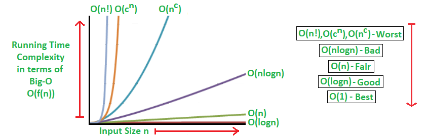
Visualization of Common Growth Rate Functions

You can see that for small input sizes they are close, but for larger input sizes they show significantly different behavior. When designing an algorithm, we want to avoid having an algorithm with exponential or factorial time complexity if possible.

Finding Big O

To prove that some function \(T(n) = O(f(n))\), we usually do not apply the definition formally but instead use a repository of known results. The results are based on the following rules:

If \(T_1(n) = O(f(n))\) and \(T_2(n) = O(g(n))\), then
- \(T_1(n) + T_2(n) = max (O(f(n)), O(g(n)))\)
- \(T_1(n) * T_2(n) = O(f(n) * g(n))\)
If \(T(x)\) is a polynomial of degree \(n\), then \(T(x) = O(x^n)\).
The base of the logarithm is not important.

In the following, we show why some of the above rules hold.

Proof of First Part of Rule 1

If \(T_1(n) = O(f(n))\) then, according to the definition, there are constants \(c_1\) and \(n_1\) such that \(T_1(n) ≤ c_1 f(n)\) when \(n ≥ n_1\).

If \(T_2(n) = O(g(n))\) then, according to the definition, there are constants \(c_2\) and \(n_2\) such that \(T_2(n) ≤ c_2 g(n)\) when \(n ≥ n_2\).

Now, let \(n_0 = max(n_1, n_2)\). Therefore:

\(T_1(n) ≤ c_1 f(n)\) when \(n ≥ n_0\)

\(T_2(n) ≤ c_2 g(n)\) when \(n ≥ n_0\)

\(T_1(n) + T_2(n) ≤ c_1 f(n) + c_2 g(n)\) when \(n ≥ n_0\)

Now, let \(c_3 = max(c_1, c_2)\). Therefore:

\(T_1(n) + T_2(n) ≤ c_3 f(n) + c_3 g(n)\) when \(n ≥ n_0\)

\(T_1(n) + T_2(n) ≤ c_3 ( f(n) + g(n) )\) when \(n ≥ n_0\)

\(T_1(n) + T_2(n) ≤ 2 c_3 max ( f(n) , g(n) )\) when \(n ≥ n_0\)

\(T_1(n) + T_2(n) ≤ c max ( f(n) , g(n) )\) when \(n ≥ n_0\) and \(c= 2 c_3\)

Proof of Rule 3

In Big-O analysis, the base of logarithm is not important. As you see in Table 1 and Figure 2, when the growth rate is a logarithmic function, we have not used any base value for the logarithm. The reason is that in Big-O analysis, the logarithm base does not matter since different bases are asymptotically the same. In other words, they differ by a constant factor because the logarithm in base b can be expressed as:

\(log_b n = log_k n / log_k b = c log_k n\)

where \(k\) is any constant number \(> 0\).

Now applying rule 1 above, we see that the constant does not matter:

\(O (log_b n) = O (log_k n)\)

Therefore, the base of logarithm does not matter.

Simplification Rules

Based on the above rules, we have the following simplification rules that are used when analyzing the algorithms.

If \(T(n)\) is constant, then we say that \(T(n)\) is \(O(1)\)
The coefficients are ignored. The constants or low-order terms are not included inside a Big-O. For example, \(T(n) = O(2n^2)\) or \(T(n) = O(n^2 + n)\) are not in correct form. Instead, in both cases, the correct form is \(T(n) = O(n^2)\). This means that in any analysis that will require a Big-O answer, we keep the fastest growing term and discard the lower terms and constants. These are the direct result of rule 1 and 2 above. For example, \(n^2 + n\) is the sum of two terms, one is \(O(n^2)\) and the other is \(O(n)\). Therefore, the larger one is chosen. Also, \(2 n^2\) is the multiplication of two terms that are \(O(1)\) and \(O(n^2)\).
If \(T(n)\) is a sum of several terms, the one with the largest growth rate is kept and all others omitted. This is direct result of rule 1 above.
If \(T(n)\) is a product of several factors, all constants are omitted. This is direct result of rule 1 above.

Tight and Loose Upper bounds

There are two other definitions that is good to know.

Definition: \(T(n) = Ω (g(n))\) if there are constants \(c\) and \(n_0\) such that \(T(n) ≥ cg(n)\) when \(n ≥ n_0\).

Definition: \(T(n) = Θ (h(n))\) if and only if \(T(n) = O(h(n))\) and \(T(n) = Ω (h(n))\).

When \(T(n) = O(f(n))\), it means that function \(T(n)\) grows at a rate no faster than \(f(n)\); thus \(f(n)\) is an upper bound on \(T(n)\). According to the above definitions, this implies that \(f(n) = Ω (T(n))\); in other words, \(T(n)\) is a lower bound on \(f(n)\).

Let's look at an example. Since \(n^3\) grows faster than \(n^2\), we can say that \(n^2 = O(n^3)\) or \(n^3 = Ω (n^2)\).

As another example, if \(f(n) = n^2\) and \(g(n) = 2 n^2\), since they grow at the same rate, both \(f(n) = O(g(n))\) and \(f(n) = Ω (g(n))\) are true. Also, we can say \(f(n) = Θ (g(n))\) or \(g(n) = Θ (f(n))\).

When two functions grow at the same rate, it could be expressed with \(Θ()\). For example, if \(g(n) = 2n^2\), then \(g(n) = O(n^4)\), \(g(n) = O(n^3)\), and \(g(n) = O(n^2)\) are all technically correct, but obviously the last one is the best answer. Writing \(g(n) = Θ (n^2)\) means not only that \(g(n) = O(n^2)\), but also that the result is a tight upper bound. In this case, \(n^4\) and \(n^3\) are loose upper bounds for \(g(n)\).

Big-O Analysis Of Algorithms

In this section, we discuss how to determine the time complexity of an algorithm. The time complexity is expressed using Big-O notation. The Big-O provides an upper bound of the runtime of an algorithm, so we need to make sure not to underestimate its runtime. In the following, first we start with a simple example, and then mention some of the rules used in general for analysis of algorithms.

Example

Let's analyze the simple program shown in Code Listing 1. It calculates the sum of numbers from 1 to \(n\). To analyze this program, first we count the number of constant time operations in terms of input size, \(n\).

Analysis of sum_of_n Function

            
def sum_of_n(n):
    partial_sum = 0        # constant-time operation (1)

    for i in range(n + 1): # initialization of sequence, traversing sequence (n)
        partial_sum += i   # constant-time operation - addition and assignment (1)
    return partial_sum     # constant-time operation (1)

The analysis of this function is simple. The function definition in line 1 takes no time. Lines 2 and 6 each are counted as one constant-time operation. Line 5 has two constant-time operations per time executed (one addition and one assignment) and is executed n times, so there are \(2n\) operations executed in total. Line 3 has \(n\) operations of initializing and traversing a sequence of values.

The initialization is done once, the test is done \(n+1\) times, and the increment is done \(n\) times, thus \(2n + 2\). Returning the function is one constant-time operation. Therefore, we have:

\(T(n) = 4n+ 4\)

Thus we say that this function is \(O(n)\).

In practice, we don't do all this work when we want to analyze a program, otherwise the task would become ridiculously difficult. Instead, we take lots of shortcuts without affecting the final answer since we are giving the answer in terms of Big-O.

For example, we do not need to count every individual constant operations. In the sample code, Lines 2 and 6 can be ignored as their execution is not significant compared to the for loop. There are several rules of thumb that we can use to find Big-O of an algorithm.

Finding Time Complexity: Rules of Thumb

When new to algorithm analysis, determining the time complexity of an algorithm can seem daunting. However, there are a few rules of thumb to go by to give you a rough idea of what an algorithm's time complexity is likely to be. The goal here is to compute Big-O efficiency. So we throw away leading constant or low-order terms as discussed before.

The runtime of a loop is at most the runtime of the statements inside the loop times the number of iterations. Specifically, in a loop that needs to process an input of size \(n\), examine the amount of data left to be processed after one iteration:

If after the first iteration the amount of data left to process is \(n-1\), this means the loop is repeated \(n\) times and the algorithm is \(O(n)\), or of linear complexity.
If after the first iteration the amount of data left to process is \(n/2\) (or \(n/k\) - the divisor doesn't matter), the algorithm is \(O(\log n)\), or of logarithmic complexity. Algorithms such as binary search have logarithmic time complexity.

Example: Linear Time-Complexity - \(O(n)\)

n = 100
for i in range(n):
    print(i)

Example: Logarithmic Time-Complexity - \(O(\log n)\)

n = 100
i = n
while i > 0 :
    i = i // 2
    print(i)

Nested Loops

The nested loops should be analyzed from the inside out. The total running time of a statement inside a group of nested for loops is the running time of the statement multiplied by the product of the sizes of all the for loops.

To be more exact and have a tight upper bound, if the algorithm has nested loops, then we need to see the amount of data left to be processed after each iteration. If there are two nested loops and if both loops are linear, then the algorithm is \(O(n^2)\) (quadratic time complexity). An example of this is when you want to visit the content of a 2-dimensional table of size n. If one loop is linear and the other is logarithmic, then the algorithm has \(O(n \log n)\) time complexity. The following is an example where the outer loop is linear while the inner loop has logarithmic time complexity:

Example: Nested while Loops

while i <= n:
    j=1
    while j <= i:
        j = j * 2
    i += 1

The inner loop has logarithmic runtime and the outer loop has linear runtime.

Example: Nested for Loops

for i in range(n):
    for j in range(i):
        a[i] += a[j]

Both loops are \(O(n)\) so the combined loops has quadratic runtime for a Big-O of \(O(n^2)\). Note although the limit of the inner loop is i and of the outer loop is n, we don't write \(O(i\times n)\) - the variable used doesn't matter, what matters is that both loops are linear, and one is nested in the other, so \(O(n^2)\) is sufficient.

Consecutive Statements

If there are consecutive statements, then their time complexity is added and lower order terms are ignored. For example, Code Listing 4 shows has an \(O(n)\) loop followed by an \(O(n^2)\) nested loop, therefore the whole code has time complexity of \(O(n^2)\):

Example: Consecutive for Loops

for i in range(n):
    a[i] = 0
for i in range(n):
    for j in range(n):
        a[i] += a[j] + i + j

A loop followed by a nested loop. The time complexity of nested loop is the dominant one in calculating the time complexity of the code segment.

Constant operations

If the algorithm has no loops or recursive calls (recursion will be discussed later in the course), then the algorithm is \(O(1)\), or of constant time complexity. The size of the data does not matter - without a loop or recursive call, the algorithm can't take more time.

General Rules

As a general rule, when analyzing a program, we need to start from the inside (or deepest part) of a program towards outer parts. If there are function calls, obviously these must be analyzed first.

Example Using the Rules of Thumb

The re-analysis of Code Listing 1, using the rules of thumb allows us to easily conclude the time complexity of \(O(n)\) and there is no need to count the exact number of operations as we did earlier.

Second Analysis of sum_of_n Function

            
def sum_of_n(n):
    partial_sum = 0        # O(1)

    for i in range(n + 1): # O(n)
        partial_sum += i   # O(1)
    return partial_sum     # O(1)

Exercise Break

How should you choose an algorithm? Is the algorithm with the lower complexity always better than the algorithm with the higher complexity? Examine the following runtime functions:

\(T_1(n) = 50000 log_2 n + 5\)
\(T_2(n) = 400 n + 20\)
\(T_3 = 3(2^n) + 6 n^2 + 0.2\)

Which of the corresponding algorithms is the best choice if \(n <\) 5? What if \(n > 1000\)?

The choice of an algorithm depends on the size of n. In this case, \(T_1 (n) = O(\log n)\), \(T_2 (n) = O(n)\), and \(T_3 (n) = O(2^n)\). Therefore, for large values of n, \(T_1(n)\) is the most efficient one. However, for small values of n, the constant coefficient matters. In this example \(T_3(n)\) is the most efficient one for values less than 5 although it has exponential running time.

Recursive Analysis

Analysis of Recursive Algorithms

We talked about analysis of algorithms in Lesson 2. We explained how the runtime is expressed as a function of input size, \(T(N)\), and how we find the time-complexity of a function using Big-O notation. In addition, we discussed how it is not required to always calculate \(T(N)\) and we can directly find Big-O of an algorithm.

Estimating the runtime of a recursive function is similar except that when we are calculating \(T(N)\), we will have function T on both sides of the equation. Therefore, we need to solve a recurrence relation. To see how it is done, we provided a number of examples in the following.

Big-O Analysis of the factorial function

Consider the factorial function shown in Figure 6. It shows how the time complexity is calculated.

Recursive Factorial Analysis


def factorial(n):
    if n == 0:                         # O(1)
        result = 1                     # O(1)
    else:
        result = n * factorial(n - 1)  # multiplication O(1) + T(N-1)
    return result                      # O(1)

As shown in the figure, the runtime function is expressed as:

\(T(N) = T(N-1) + c\)

The above equation is not enough to find the growth rate and we need to solve the recurrence relation. One technique to derive \(T(N)\) is to expand the right side and count the number of constant factors:

\(T(N) = T(N-1) + c\)
\( = T(N-2) + c + c = T(N-2) + 2c\)
\( = T(N-3) + c + c + c = T(N-3) + 3c\)
\( = ... \)
\( = T(0) + Nc = O(n)\)

Big-Oh Analysis of the fibonacci function

The following figure shows how the \(T(N)\) is calculate in fibonacci function.

Recursive Fibonacci Analysis


def fibonacci(n):
    if n <= 0:                                        # O(1)
        result = 0                                    # O(1)
    elif n < 2:                                       # O(1)
        result = 1                                    # O(1)
    else:
        result = fibonacci(n - 1) + fibonacci(n - 2)  # addition O(1) + T(N-1) + T(N-2)
    return result                                     # O(1)

After the above step, we get the following recurrence relation to be solved:
\(T(N) = T(N-1) + T(N-2) + c\)

To solve the above recurrence relation, we replace \(T(N-2)\) by \(T(N-1)\), so that it is easier to find \(T(N)\). Therefore, what we find is an upper bound on runtime function since \(T(N-2) <= T(N-1)\)

Therefore, the runtime function would be:

\(T(N) = 2 T(N-1) + c\)
\(= 2 (2 T(N-2) + c) + c = 4 T(N-2) + 3c\)
\(= 4 (2 T(N-3) + c) + 3c = 8 T(N-3) + 7c\)
\(= 8 (2 T(N-4) + c) + 7c = 16 T(N-4) + 15c\)
\(= 16(2 T(N-5) + c) + 15c = 32 T(N-5) + 31c\)
\(= ...\)
\(= 2^{N-1} T(1) + (2^{N-1} - 1) c\)
\(= 2^{N-1} + 2^{N-1} c - c\)
\(= 2^{N-1} (1 + c) - c\)

Therefore,

\(T(N) = 2^{N-1} (1 + c) - c = O(2^n)\)

It shows that the fibonacci algorithm has an exponential running time and it is not efficient. We already discussed why this algorithm is not efficient as it involves repetitive calls to evaluate the same value. Here, using algorithm analysis we showed that this algorithm is not efficient.

If we estimate the time-complexity of the iterative fibonacci function in Section 8.4.2.1, we see that:

\(T(N) = c + (N-2) * c = O(n)\)

Therefore the iterative Fibonacci is much faster than the recursive one.

Summary

In this lesson, we discussed how to estimate the time used by an algorithm. We mentioned the limitations with experimental measurement and discussed a theoretical approach for estimating the time used by an algorithm called asymptotic analysis. The time estimated by this approach is called time complexity and is computed using Big-O notation. It is a measure of how the algorithm behaves when the input size is increased. The Big-O notation tells us which algorithm is preferable for large values of n . If the size of the input data is always very small, then Big-O notation may not necessarily tell you which algorithm is the best choice.

Although in this lesson we focused on time-complexity of an algorithm, the memory usage of an algorithm, space-complexity, could be estimated similarly using asymptotic analysis as a function of input size. We will see examples of that as we go through the course.

Usually there are different operations available on data structures/ADTs and those operations could be done using different algorithms. The goal is to perform the operations on data efficiently. To compare the efficiency of algorithms in terms of time and space, we will repeatedly refer to the techniques introduced in this lesson.

References

Wikipedia: Algorithmic efficiency
Design and Analysis of Data Structures, Niema Moshiri and Liz Izhikevich, 2018.
Data Structures and Algorithm Analysis in C++, Mark Allen Weiss. 2006.
MIT 6.00SC | Lecture 08 | Efficiency and Order of Growth