Topics

In this lesson, we are going to introduce recursion. Topics include:

1. The concept of recursion
2. Using recursion in programming
3. The execution process of recursive functions
4. Uses of recursion in problem solving
5. The analysis of recursive algorithms

Required Tasks

1. Read this lesson.
2. Complete Lab 5.
3. Complete and submit Assignment 8.

Learning Outcomes

By the end of this lesson, you should be able to

1. Define the concept of recursion.
2. Articulate the difference between iterative and recursive solutions.
3. Explain how a recursive algorithm is executed on a system.
4. Develop the code to solve problems using recursion.
5. Estimate the time-complexity of a recursive algorithm.

Introduction

In this lesson, we will be talking about recursion. Recursion means defining something in terms of itself. Something that is defined using recursion is defined recursively. We will be talking about using recursion in defining data structures and mathematical functions. Recursion is also used in different programming language to develop recursive functions. Moreover, recursion is used as a programming technique to solve problem. Finally, we discuss the time-complexity of recursive functions.

Recursion

Mathematical Recursion

Many mathematical functions are defined using recursion. A function that is defined in terms of itself is called a recursive function. For example, factorial function:

\(f(n) = n! = n \times (n-1) \times ... \times 1\)

could be define recursively:

\(f(0) = 0! = 1\)   (base case)

\(f(n) = n \times f(n-1)\) for \(n >= 2\)

The first line defines the base case; that is, the value for which the function is directly known without resorting to recursion. The case where the function calls itself is the general case.

Recursive Functions

Recursion is also used as a technique in programming where a function calls itself to solve a problem. The function that calls itself is called a recursive function. Python like many other languages allow functions to be recursive.

Consider the code of factorial function given in the following Listing. The factorial is undefined for a negative number. Let's see what happens as a result of calling factorial(-1).

def factorial(n) :
  if n == 0:
    result = 1
  else:
    result = n * factorial(n - 1)
  return result

It is important that recursive calls are made in such a way that the calls move towards the base case. Trying to evaluate factorial(-1) results in calls to factorial(-2), factorial(-3), and so on. Calling factorial(-1) never gets to a base case and the program will not be able to find the answer (which is undefined anyway). This is an example of infinite recursion. (The reality is that, unlike an infinite loop, infinite recursion is usually not truly infinite, as the computer runs out of memory and the function dies.)

Rules of Recursion

The previous examples lead us to the rules of recursion that must be followed when defining a recursive function:

1. Every recursive function must have at least one base case: a condition under which no recursive call is made and the recursion stops. In this case, the recursive function returns the result without resorting to the recursion.
2. The function must have at least one condition where a recursive call occurs. The recursive calls must always be to a case that makes progress towards a base case. The function must have the possibility of reaching the base case, or it ends up with infinite recursion.

The basic structure of a simple recursive function looks something like this:

        
def recurse(value):

    if {base case condition is true}:
        # Base case - recursion stops.
        ans = {base case value}
    else:
        # General case - make recursive call.
        ans = {general value} + recurse({changed value})
    return ans

      

There are countless variations on this, but the basic approach is the same.

How Recursion Works

The details recursion works 'under the hood', so to speak, are beyond this course, but covered in great detail in CP216: Introduction to Microprocessors. However, we can provide a brief discussion and a visualization that you can try for yourself.

In a computer's memory, every function call is pushed onto an execution stack. When the execution of a function is finished, it is popped off the stack and its return value(s) sent back to the calling function or program, which is also on the execution stack. The execution stack grows as more functions are called, and shrinks as they finish. Recursive calls are different from standard function calls only in that they call copies of themselves with different parameter values.

The Python Tutor visually shows a function stack as a recursive function is executed (you can try this yourself):

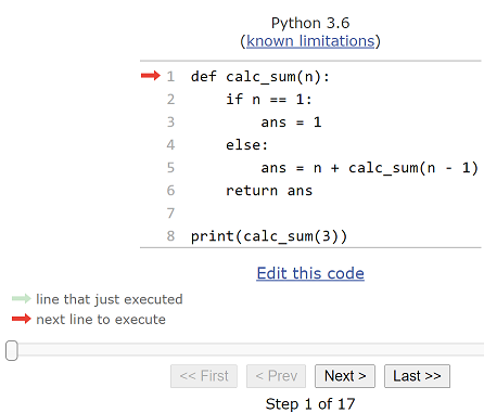
The function is defined and we can now step through its execution with .

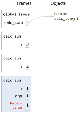
We have pressed until reaching the base case. At each press of the button a call to calc_sum is added to the stack of function calls (the top is at the bottom of the image) with the value of n at each call. In the last call (the base case call) at the top of the function stack, n is 1 and the return value is 1, which is the base case return value.

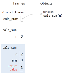
The base case call has returned 1 to its parent call, which now adds that result to n of 2 for a return result of 3. (Based on the line ans = n + calc_sum(n - 1))

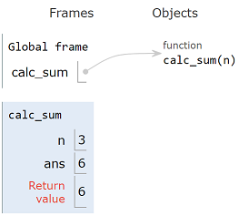
The function call adds its n of 3 to the return value 3 of its recursive call for a total of 6.

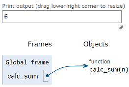
The final value of 6 is returned to whatever called the calc_sum function in the first place.

Recursive Algorithms

A recursive algorithm solves a problem by applying its algorithm to a series of 'smaller' problems. The smaller solutions add up to the bigger solution. An example of a recursive algorithm is finding the meaning of a word in a dictionary, where words are defined in terms of other words:

• If we know the meaning of a word, then we are done (base case)
• Otherwise, we look the word up in the dictionary. If we understand all the words in the definition, we are done; otherwise, we need to figure out what the definition means by recursively looking up the words we don't know. This procedure terminates if the dictionary is well defined but terminates badly if a word is either not defined, or recurses indefinitely if a word is circularly defined. For example:
  

  Circular Definition: a definition that is circular.

  Recursion: something that uses a recursive algorithm
  Recursive Algorithm: an algorithm that uses recursion

Recursion vs Iteration

If recursion has so many drawbacks, why use recursion at all? You can (for the most part) write any iterative (looping) algorithm as a recursive algorithm, but the reverse is not necessarily true, or at least not without using space resources greater than those the recursive algorithm would use by default. Recursion is an alternative to iteration, and it is a very powerful problem-solving technique. The recursive algorithm may also be significantly simpler than its equivalent iterative algorithm, and therefore simpler to write. We will see that this is often the case when working with certain kinds of linked data structures.

Solving Problems Using Recursion

In the following we discuss a few examples where recursion makes an algorithm clearer than an iterative version might.

Calculating Fibonacci Numbers

Fibonacci Numbers are the number of this sequence:

1, 1, 2, 3, 5, 8, 13, 21, 34, 55, 89, …

We can define these numbers recursively:

\(fib(1) = 1\)
\(fib(2) = 1\)
\(fib(n) = fib(n – 1) + fib(n – 2)\) for \(n > 2\)

def rfib(n):
    assert n >= 1
    if n == 1 or n == 2:
        result = 1
    else:
        result = rfib(n - 1) + rfib(n - 2)
    return result

def ifib(n):
    if n == 1 or n == 2:
        result = 1
    else:
        prev = 1
        current = 1
        result = 0
        for i in range(3, n + 1, 1):
            result = prev + current
            prev = current
            current = result
    return result

Comparing the recursive version versus the iterative version, we see that the recursive version is easier to understand and it is shorter, simpler, and closer to the 'math' definition of the Fibonacci algorithm.

Now, let's compare the efficiency. In addition to the overhead associated with the execution stack, there are many repetitive calls in the recursive version. The follwoing Figure shows the function calls made for calculating rfib(6). As you see, to evaluate rfib(6), rfib(4) is called twice, rfib(3) is called three times, rfib(2) is called five times and so on. There are many repetitions involved and that leads to the inefficiency in this algorithm. The iterative version has more variables and is less clear, but it avoids repetitive calculations.

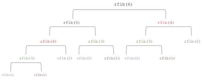
Created by Masoomeh Rudafshani. Used with permission.

Towers of Hanoi

A classic example of a problem that is solved easier using recursion is the Towers of Hanoi puzzle. It consists of three rods and several discs of different sizes that can slide into any of the rods. Initially the discs are placed on one rod in ascending order of size; i.e., the largest disc on the bottom and the smallest one on top as shown in the following Figure:

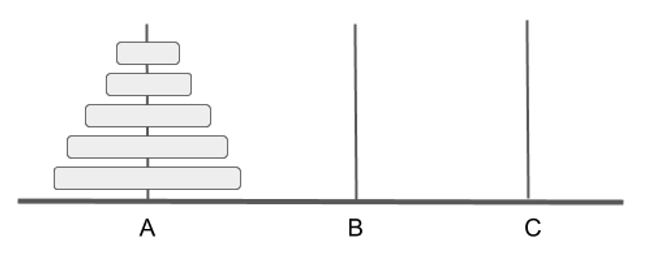
Created by Masoomeh Rudafshani. Used with permission.

The goal of this puzzle is to move all of the discs from the leftmost rod to the rightmost rod. It is OK to use the middle rod, but the moves should be according to the following rules:

• Only one disk can be moved at a time
• During a move, the upper disc from one of the rods is placed on top of another disc or on an empty rod. Only one disc is moved at a time.
• A disk cannot be placed on top of a smaller disk

Recursive Algorithm

Here is the algorithm to move a stack of n disks from the leftmost rod to the rightmost rod:

1. If there is just one disc (the base case), then move the disc from leftmost rod to the rightmost rod
2. Otherwise:
   • move the topmost n-1 disks from the leftmost rod to the middle rod
   • move the largest disk from the leftmost rod to the rightmost rod
   • move the n-1 disks from the middle rod to the rightmost rod

The following Listing, shows an implementation of a recursive function to solve the Towers of Hanoi puzzle.

def Hanoi(leftRod, rightRod, midRod, n):
    if n == 1:
        print(f"Move disk from {leftRod} to {rightRod}")
    else:
        Hanoi(leftRod, midRod, rightRod, n - 1)
        print(f"Move disk from {leftRod} to {rightRod}")
        Hanoi(midRod, rightRod, leftRod, n - 1)

Hanoi("A", "C", "B", 3)

Move disk from A to C
Move disk from A to B
Move disk from C to B
Move disk from A to C
Move disk from B to A
Move disk from B to C
Move disk from A to C

If you run the code in Code Listing 3, you will see that the number of moves increases exponentially as the number of disks increases: for 1 disk there is one move, for 2 disks there are 3 moves, for 3 disks there are 7 moves, for 4 disks there are 15 moves and for 5 disks there are 31 moves, and so on. Therefore, the time-complexity of this algorithm is exponential: \(O(2^n)\).

Types of Recursion

Our examples so far have involved working with integer parameters. Data structures can also be manipulated recursively. A recursive data structure is a structure that can be defined in terms of itself.

Recursion on Strings

A string can be defined recursively:

• Empty space is a string (base case)
• A string is a character followed by a string (general case)

The function in Code Listing 1 reverses a string recursively. The key to understanding this function is in the recursive call. Every time the function calls itself, it passes a smaller and smaller part of the string as an argument to the recursive call. (In Python the string slice operation s[1:] returns an empty string rather than an error when only one character is left in the string.

def string_reverse(string):
    if string == "":
        new_string = ""
    else:
        new_string = string_reverse(string[1:]) + string[0]
    return new_string

Recursion on Lists

Python lists, and thus the ADTs based on lists we've developed earlier in this course could also be manipulated recursively. One approach to reversing a list looks a great deal like reversing a string:

def list_reverse(items):
    if items == []:
        new_items = []
    else:
        new_items = list_reverse(items[1:]) + [items[0]]
    return new_items

This is not the only way to reverse the contents of a list recursively, but it is the only way to do so with a string. Some data structures allow different types of recursion to be applied to them.

Fruitful Recursion

In fruitful recursion, the recursive function returns one or more values. This is nothing new to us - we have written many functions that return something. In the context of recursion, however, this means that the recursion relies on the fact that each recursive call returns a value used in the recursion. Both Code Listing 1 and Code Listing 2 show examples of fruitful recursion.

The following is another approach to reversing a list using fruitful recursion:

def swap(items, i, j):
    temp = items[i]
    items[i] = items[j]
    items[j] = temp
    return

def list_reverse_fr(items):
    n = len(items)

    if n > 1:
        swap(items, 0, n - 1)
        items[1:n - 1] = list_reverse_fr(items[1:n - 1])
    return items

This function reverses the contents of a Python list by changing slices of the list. This function uses the swap function to 'swap' two elements of a list. The function first determines whether or not there are enough elements to swap - a list must have at least two elements in it to perform a swap. It then updates the interior of the list (i.e. everything except the first and last values of the list) with the result of the recursive call. An ever smaller list is passed to the recursive call, guaranteeing that eventually the base case will be reached. Because the function returns a value it is a fruitful function, and because the function is fruitful the result of the function must be used or the changes to the list are lost.

The following diagram shows how the fruitful recursion is handled:

In-Place Recursion

In-place recursion uses functions that generally do not return values, rather they manipulate the contents of the data structures they use in-place. The list_reverse_ip function shows an example of reversing the contents of a Python list by swapping the elements of the list in-place.

def list_reverse_ip(items, m, n):
    if n > m:
        swap(items, m, n)
        list_reverse_ip(items, m + 1, n - 1)
    return

x = [1, 2, 3, 4, 5]
list_reverse_ip(x, 0, len(x) - 1)

This function takes the indexes of the first and last elements in items as its parameters along with a references to items itself. The base case thus relies on the relative values of the n and m indexes: as long as there are values left to swap, the function swaps them. Each recursive call passes the same reference to items and moves n and m closer together. The function does not return a value, and is therefore not fruitful.

The following diagram shows how the in-place recursion is handled:

It is worth noting that this function uses less storage space than the previous one. In list_reverse_fr when the list segment is passed to each call of the function, Python actually passes a copy of that segment of the list. In list_reverse_ip the function passes a reference to the location of the entire list in memory, and this reference never changes (thus the 'in-place' name). As lists grow large, the amount of stack space needed to copy list segments gets very large as well.

Note further that list_reverse_ip requires more information than list_reverse_fr when first called, i.e. the indexes of the first and last values of the list. However, we'd like to be able to pass only the list itself as a parameter to match the parameter of the fruitful function. How to do this is covered in the next section.

Tree Recursion

Tree Recursion is defined as recursion in which there are potentially multiple recursive calls within a function, thus forming a 'tree' of recursive calls. The Fibonacci and Towers of Hanoi functions shown earlier are examples of tree recursion. Note that tree recursion may either be fruitful or in-place.

Tree recursion is often used with tree data structures such as the Binary Search Tree (BST), to be covered in a later section.

Which Recursion Should I Use?

Which approach should you use? The type of recursion that can be used depends not only on the algorithm, but may be language dependent. For example, strings in Python are immutable, and because they are immutable their individual elements cannot be swapped in-place. Thus a recursive function to reverse a string must be fruitful. Other languages may not provide the equivalent of list segments and therefore must use an in-place algorithm. As we will see when using tree data structures, tree recursion may be an easy-to-understand and elegant solution to a problem.

Auxiliary Functions

In this section, we are going to discuss how using auxiliary functions allows us control over the parameters passed to a recursive function.

Defining Auxiliary Functions

The definition of the list_reverse_ip function required parameters beyond that of just a reference to the list to reverse. This not only puts a burden on the programmer, but because the indexes pass are always the indexes of the first and last values in the list, it would be easier to use if these extra parameter were not necessary. The solution is to use an auxiliary function as in the following example:

def list_reverse_ip(items):
    list_reverse_ip_aux(items, 0, len(items) - 1)
    return


def list_reverse_ip_aux(items, m, n):
    if n > m:
        swap(items, m, n)
        list_reverse_ip_aux(items, m + 1, n - 1)
    return

x = [1, 2, 3, 4, 5]
list_reverse_ip(x)

In this code the auxiliary function list_reverse_ip_aux (in this course, the _aux ending is typically given to an auxiliary function to make it clear that the function is indeed an auxiliary function), performs the actual recursion. Now the only job of the base function list_reverse_ip is to call its auxiliary function and provide that function with the necessary extra parameters. list_reverse_ip is still considered to be an recursive function despite the fact it is not recursive itself, but it does rely on a recursive auxiliary function to do its work.

Defining Auxiliary Methods

In general, auxiliary functions are required any time we require access to extra or different parameters that are either inaccessible to the base function, or would be clumsy to use. We don't, for example, have access to the private attribute _values in our array-based data structures from outside those data structures, so we couldn't refer to len(stack._values) if we wanted to reverse the contents of a Stack recursively. We could, however, pass len(self._values) as a parameter to an auxiliary method defined inside the Stack class module Stack_array.py, as in the following example:

class Stack:

    def reverse(self):
        self._reverse_aux(0, len(self._values) - 1)
        return

    def _reverse_aux(self, m, n):
        if n > m:
            temp = self._values[m]
            self._values[m] = self._values[n]
            self._values[n] = temp
            self._reverse_aux(m + 1, n - 1)
        return

# Sample call
stack = Stack()
# add values to stack
stack.reverse()

Note that the auxiliary method does not need the list _values as a parameter. As a Stack method it has direct access to all of the Stack attributes, thus the reference to self._values. The auxiliary method is also named with a leading _ (underscore) to indicate that the method is private. Nothing from outside the Stack definition should ever call a Stack auxiliary method directly.

(This could also be easily done with an iterative method - this is shown just as an example of data structure recursion.)

Note that if you write an auxiliary function or method that uses the same number and type of parameters as the base function or method that calls it, then you probably don't need the auxiliary function - or you wrote it incorrectly.

Using auxiliary functions for recursion, particularly with data structures, is a very common technique that you must master.

Summary

In this lesson, we talked about recursion in general. We explained how recursion could be used in problem-solving and programming. To develop a recursive function, make sure to have the correct base case(s). In addition, each call must move towards the base case. We explained how a recursive function works. In addition, we showed that recursion could simplify the code of a program; however, it could lead to inefficiency in terms of time and space. As you saw in the recursive Fibonacci, the recursive implementations generated large numbers of calls (many of them were repetitive).

There are different techniques for developing a recursive function. A recursive function might call itself several times (tree recursion). In addition, a recursive function that performs on a data structure might return and replace part of the data structure on each recursive call (fruitful recursion), or just change the content of a data structure (in-place recursion). Note that the tree recursion may either be fruitful or in-place. Not all recursive algorithms can be implemented using all different techniques, and the ability to do so is sometimes language dependent. For example, strings in Python are immutable, and because they are immutable their individual elements cannot be swapped in-place. Thus a recursive function to reverse a string must use fruitful functions.

References

1. Data Structures and Algorithm Analysis in C++, Mark Allen Weiss. 2006.
2. CSE373: Data Structures and Algorithms, School of Computer Science and Engineering at University of Washington, Notes on Queue ADT, https://courses.cs.washington.edu/courses/cse373/02sp/lectures/
3. CS1027b: Computer Science Fundamentals II, Department of Computer Science at Western University, Notes on Recursion, https://www.csd.uwo.ca/courses/CS1027b/
4. CS367: Introduction to Data Structures, Department of Computer Science, University of Wisconsin-Madison, Notes on recursion, http://pages.cs.wisc.edu/~hasti/cs367-1/