Topics
In this lesson, we are going to study Hashing, and in particular the Hash Set. Topics include:
- Hashing concepts
- Hash Set insertion, deletion, and traversal
Required Tasks
- Complete and submit the tasks of Lab 9.
- Complete and submit the tasks of Assignment 9.
Learning Outcomes
By the end of this lesson, you should be able to:
- Understand the concepts behind Hashing.
- Implement various Hash Set methods.
Hashes
We've seen various data structures for storing and retrieving data. Linear lists provide \(O(1)\) insertion and \(O(n)\) searching, binary search trees provide \(O(\log n)\) (average case) insertion and retrieval. Can we do better in terms of time complexity for insertion and retrieval? Yes, it turns out that we can, using hashing. There are a number of different ways of using hashing, but we will look only at the Hash Set data structure.
Hashing is implemented by a hash function, a function that, given a key value, returns an integer value. We can then use this integer value to decide where in a storage array the data should be stored. Ideally each key value generates a unique index value, thus placing each piece of data in a separate and unique location in the data array. In practice we have to be able to deal with situations where different key values generate the same index value, which we will look at later.
Using Movie data as an example, we know that Movie
objects use their title and year as a key, i.e. these are the values
used by the __eq__ method to compare Movie objects. A hash
method converts those two attributes into an integer number. To do this
we are going to extend the Movie class by implementing a
magic __hash__ method. (Python then allows you to call this
method with the keyword hash.) The __hash__
method must turn the Movie title and year into an integer. The following
method does just that:
    def __hash__(self):
        """
        -------------------------------------------------------
        Generates a hash value from a movie title and year.
        Use: h = hash(movie)
        -------------------------------------------------------
        Returns:
            returns
            value - the total of the characters in the title string
            multiplied by the year (int > 0)
        -------------------------------------------------------
        """
        value = 0

        for c in self.title:
            value = value + ord(c)
        value *= self.year
        return value
(The ord function returns the integer code version of a
character.)
Applied to some of our Movie data, this hash function produces values such as:
| Movie Key | Hash |
|---|---|
| "I Am Legend", 2007 | 1810314 |
| "Dark City", 1998 | 1652346 |
| "Omega Man, The", 1971 | 2306070 |
| "Zulu", 1964 | 848448 |
Note that this hash function is arbitrary. It could have added the character codes together rather than multiplying them, for example. Designing good hash functions - ones that, given a certain set of data, is most likely to limit repeated values - is a entire area of study that we will not get into.
Note that hash values don't have to be so complex to calculate. A Student, for example, has an integer ID that could be used directly as a hash value with no further calculations needed.
Direct Access Tables
Direct Access Table Concepts
To have a data structure with constant time for insert, find, and delete operations, the first idea is to store the data elements in an array. More specifically, if the keys are unique and integer numbers in the set \(U = {0, 1, ... m-1}\), then, we can store each data element at the array location \(T[key]\). \(T\) is the array used to store data and is called a table. Each position, or slot, in the table corresponds to a key in the universe \(U\) of all possible keys. Slot \(k\) stores the data element with key \(k\). There is where hashes can play a part, because a hash value can be used as a key.
The size of array is chosen so that it covers all possible hash values. This idea takes advantage of the fact that we can do a sub-scripting operation on an array in constant time. Figure 1 shows an example where keys are integer numbers between 0 and 10, and an array of size 11 is used to store data elements.
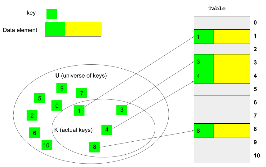
Each data element is placed in the position that is the same as its hash key.
Created by Masoomeh Rudafshani. Used with permission.
Using a direct access table, the three main operations, insert, find, and delete, can be implemented easily as shown in Code Listing 1. These operations are trivial and each takes constant time O(1) in the worst-case scenario. An alternative implementation of direct access table would be to store a pointer to the data element in the direct access table rather than the data element itself as shown in Figure 2. An empty slot points to None.
    def insert(self, v):
        self.table[hash(v)] = v
        return

    def find(self, v):
        return self.table[hash(v)]

    def delete(self, v):
        self.table[hash(v)] = None
        return
Direct Access Table Limitations
The direct access tables provide \(O(1)\) time for insert, find, and delete operations in the worst case. However, there are some limitations with this approach:
- The largest possible key (the largest value in the universe of keys, U) may be very large and it may be impractical to store a table of size \(|U|\). For example, it is impractical to store the information of all the students of a university in an array. If the student IDs have 10 digits, that means we need an array of size \(10^{10}\) to store each student's information in an array position.
- The number of elements actually stored in the Table may be small relative to the number of all possible keys (\(|U|\) much greater than \(|K|\)). In this situation, storage in the table would be very sparse and so much space would be wasted. Suppose in the example shown in Figure 1, the range of keys are 0 to 99999, but the actual keys are the one shown in these figures. It means that we need to allocate an array of size 100000 while only 4 cells are used.
- All of the keys must be unique, and unless we are using data like Student data which guarantees that no two Students have the same ID key, we may have cases where two values hash to the same table location.
To solve the above problems and at the same time have fast operations, we use a hash table. Similar to direct access tables, hash tables use an array for storing the data elements. However, there are more details to make it possible to solve the problems above, yet still have a fast data structure. In the following section we discuss the details of a hash table data structure.
Hash Tables
Hash Table Concepts
A hash table is data structure that contains an array with fixed size, called a table. Each position in the table is called a slot or a bucket. The size of a hash table, which is actually the size of the array, is its capacity. A hash table's capacity is generally much smaller than the number of all possible key values (\(|U|\)) in the data it stores.
To insert a data element into a hash table, first the key is mapped into some number in the range 0 to capacity - 1. This mapping is done using the integer key (i.e. the hash) of a value modulus (%) the capacity of the hash table. We can then use the resulting number decide where in the hash table the value should be stored. You can think of this as a two-step hash process. The hash function of a Movie object, for example, does not, and should not, know the size of a hash table's array. The first step, then is to get the integer key of a Movie object by calling its hash method, then modifying that key so it fits within the hash table's array capacity with a second hash where we apply the modulus to the value's key.
In other words the modulus maps the universe \(U\) of keys into the slots of a hash table:
f(U, capacity) → {0 … capacity - 1}
Figure 1 shows an example where keys are integer numbers in a wide range. In such a situation, if we use a direct access table, we would end up with a large array that is mostly empty since the number of keys are small. However, using a hash table, we use a much smaller array to store the data elements. A data element is placed in the position specified by the hash value of its key.
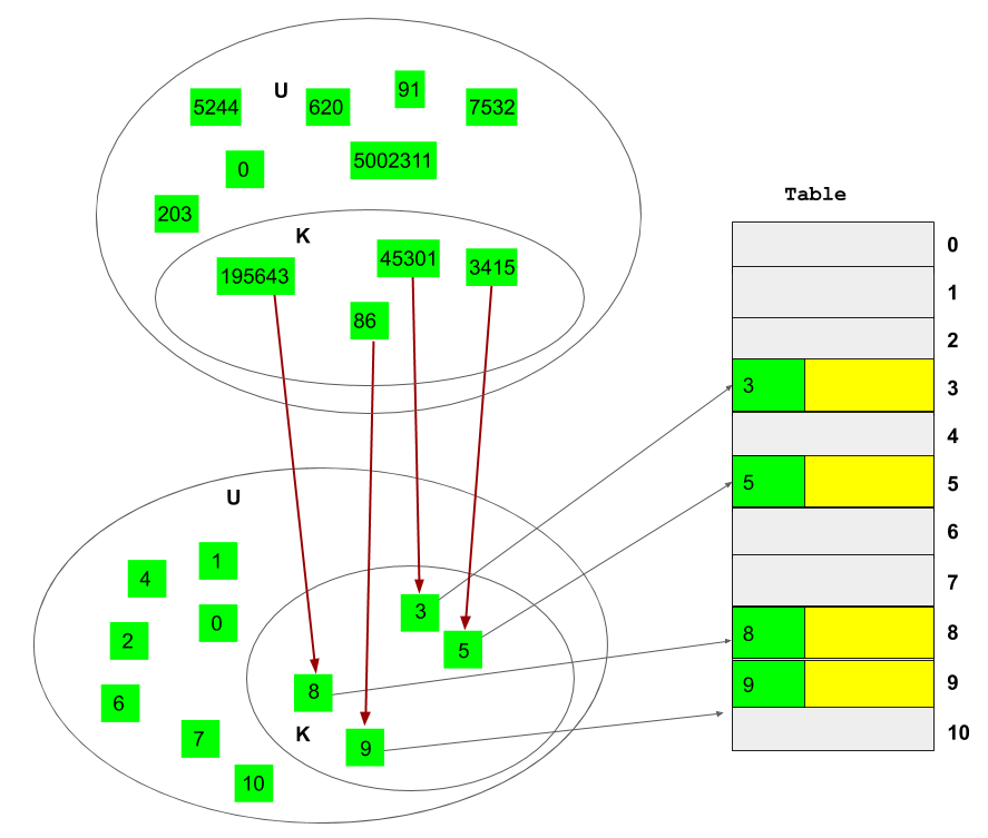
The key mapping here is \(hash(v) \bmod 11\)
Created by Masoomeh Rudafshani. Used with permission
In a hash table, we can insert, find, and delete data elements based entirely on hash values. In order to find a data element, we calculate the hash value of its key, and immediately find the location of that data. Because we use only hash values, a find method is comparison-less. We no longer have to do a search through a data structure by comparing data elements at each step. To insert a data element, we calculate the hash of its key and place the element in the position returned by the hash function. To delete a data element, we calculate the hash of its key and then make the position returned by the hash function to be None.
Note that the above operations are efficient if the hash function used is efficient. Whenever we say constant time we mean it independent of the hash function used. The explanation is that a hash calculation depends on the key value, not on the number of data elements stored in the data structure. The time required for any given hash calculation is unchanged whether the number of data elements in the data structure (\(n\)) is halved or increased by ten times.
So far, we have introduced the basic idea of hashing. There are some design decisions that need to be addressed; they result in different implementations of hash tables:
- The choice of the hash function is important. The hash function should be simple to compute and should be fast, otherwise it affects the runtime of operations on hash tables. In addition, since the number of slots in the table is smaller than the number of keys, two keys may hash to the same value. Therefore, it is impossible to place every data element in a separate location in the table array. Therefore, a good hash function should distribute data elements uniformly and uniquely among all positions in the table.
- The situation when two keys hash to the same value is known as a collision and will be addressed through collision resolution strategies. Poor hash functions can make this problem worse.
- Collisions can easily happen if the number of slots is small or the hash value is small compared to the number of data slots. Therefore, the capacity of the table is also important. Some hash functions work best when the data storage size is a power of 2, others when the storage size is a prime number. To reduce the collision, the size of the table and the hash function go hand in hand.
The following table shows how sample Movie data is distributed amongst a hash table of seven slots:
| Movie Key | Hash | Index (%7) |
|---|---|---|
| "I Am Legend", 2007 | 1810314 | 2 |
| "Dark City", 1998 | 1652346 | 3 |
| "Omega Man, The", 1971 | 2306070 | 4 |
| "Zulu", 1964 | 848448 | 6 |
| "Last Man On Earth, The", 1964 | 3609832 | 2 |
| "Dellamorte Dellamore", 1994 | 3952108 | 6 |
We see in this example that there are two collisions (the red and blue indexes) between Movies. In the next section we'll see how to resolve this problem.
Hash Table Limitations
Given how data is split up amongst different slots, insertion, removal, and searching is very efficient, but operations such as finding the minimum and maximum are very difficult because each slot has to be searched for a minimum or maximum separately and that value compared against the minimum or maximum found so far. Retrieving data in sorted order would be even more difficult even if the individual slots were sorted.
Collisions
Handling Collisions
There are a number of different methods for dealing with collisions in a hash table, such as linear probing, quadratic probing, and double hashing. We will look in detail only at separate chaining, which has the advantage both of simplicity and taking advantage of other data structures we have already created.
Separate Chaining
In this technique to solve the collision problem, each slot in the hash table points to a data structure (e.g. a list, sorted list, or binary search tree) to store multiple data elements that hash to the same slots in the table. There could be as many as lists in the hash table as its capacity. The resulting hash table is referred to as a chained hash table. This strategy is shown in Figure 4.
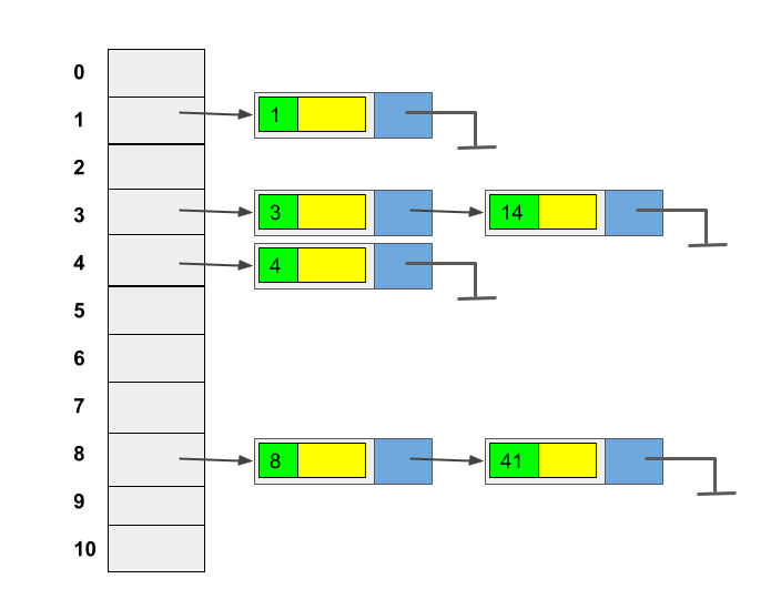
Each slot in the table pints to a linked list data structure. The hash function is: \(h(k) = k \bmod 11\)
Created by Masoomeh Rudafshani. Used with permission.
To insert a data element into a chained hash table, we first find the hash value of its key, which specifies the slot in the table to store the data element. We then go to the List assigned to that slot and attempt to insert the element into that List. If the data element already exists in the List, we reject it. Otherwise it is added to that List. This may require a search upon the List in that slot, but we can ignore all the other slots. Further, that List can grow as large as necessary to accommodate as many items as we like. To find a data element, we apply the hash function and search within the List. Deleting is similar: after finding the appropriate List, we delete the element from the list.
Big-O Analysis of Separate Chaining
In the worst-case scenario, all our hash values converge to the same slot, and we end up with a simple List. (The result is similar to the problem that occurs when values are inserted in order into a BST, but the cause is very different.) In the best scenario, colliding items are spread out evenly amongst the various Lists in the array slots.
To analyze the hashing with separate chaining, we first define the load factor of a hash table. Let \(n\) be number of items to be stored in a hash table and \(m\) be the number of hash table slots. The load factor, \(λ\), is defined to be \(n/m\). For example, if \(m=101\) and \(n=505\), then \(λ=5\); if \(m=101\) and \(n=10\), then \(λ=0.1\).
Worst-Case Scenario
In the worst case all \(n\) keys hash to the same slot, creating a list of length \(n\). Therefore, the find operation takes \(O(n)\). The insert is \(O(1)\) if we insert at the beginning of the List assigned to a slot. However, if a data element is inserted only if the key does not exist (in a set, for example), then we need to do a search first. In this case, insert would be \(O(n)\). The delete is \(O(n)\) since we need to first find the element.
Average-Case Scenario
The average length of a linked-list is \(λ\). Therefore, average time for accessing a data element would be \(O(1)+O(λ)\). To have constant time, we need to keep \(λ\) close to 1 (i.e. \(m≈n\)). If we have a simple uniform hash function and the size of the table is reasonable (not too small compared to the number of data element), every key is equally likely to hash to any of the \(m\) slots and the load factor would be constant. Therefore, the operations would run in constant time.
Separate Chaining Limitations
The chained hash tables have some disadvantages:
- It is necessary to implement and use a second data structure; for example, a linked List as discussed here.
- This second data structure, whatever it is, imposes extra costs for its use in insert, deletion, and searching.
Rehashing
Rehashing in Separate Chaining
When working with hash tables, at some point it may be useful to increase the number of available slots instead of continuing to grow the Lists attached to the slots. The decision on when to do this is based upon the load factor.
The load factor - the word factor is used deliberately because it is part of a calculation, not a limit value - is used together with the Hash Set capacity to calculate the maximum number of values that can be stored in a Hash Set before it needs to be rehashed. The formula is:
maximum values in hash table before rehash = capacity × load factor
Thus, if the current capacity is 7 slots and the load factor is 20, then the Hash Set can hold up to 140 items before the set must be rehashed. The number of items in any single slot is irrelevant, and potentially inefficient. Imagine a rehash based upon some maximum slot size. You get 21 items in a slot, you rehash, and at the end of the rehash a different slot has 21 items – so you rehash immediately. And another slot ends up with 21 items, so you rehash immediately, etc… This is not efficient or useful.
Rehashing Algorithm
In a rehash, the number of available slots in a hash table is increased. The number of slots could be doubled, for example. To rehash, first, a new table is created which has a capacity larger than that of the original table. Then, all of the data elements in the hash table must have their indexes recalculated and be moved to a new slot. We cannot just copy data elements from the old table to the new table because the hash function and the number of slots have changed and therefore the indexes associated with the key may change as well.
Rehashing can be done as often as necessary as the hash table grows.
Rehashing Example
Let's revisit our Movie data stored in a hash table of 7 slots:
| Movie Key | Hash | Index (%7) |
|---|---|---|
| "I Am Legend", 2007 | 1810314 | 2 |
| "Dark City", 1998 | 1652346 | 3 |
| "Omega Man, The", 1971 | 2306070 | 4 |
| "Zulu", 1964 | 848448 | 6 |
| "Last Man On Earth, The", 1964 | 3609832 | 2 |
| "Dellamorte Dellamore", 1994 | 3952108 | 6 |
Assume that adding a new Movie exceeds the load factor × capacity for the hash table and the table is forced to rehash. The capacity of the table is recalculated as \(capacity=2\times capacity + 1\). (Capacities that are odd in size or based upon prime numbers are more efficient for reasons too esoteric to get into here.) The existing Movie values all have new indexes calculated and are moving into the new, larger, table using \(k\bmod 15\). The resulting table is:
| Movie Key | Hash | Index (%15) |
|---|---|---|
| "I Am Legend", 2007 | 1810314 | 9 |
| "Dark City", 1998 | 1652346 | 6 |
| "Omega Man, The", 1971 | 2306070 | 0 |
| "Zulu", 1964 | 848448 | 3 |
| "Last Man On Earth, The", 1964 | 3609832 | 7 |
| "Dellamorte Dellamore", 1994 | 3952108 | 13 |
| "Wrong Box, The", 1966 | 2396554 | 4 |
Analysis of rehashing in open hash table
The runtime of rehashing is \(O(n)\), since there are n elements to rehash. However, since it happens very infrequently the amortized complexity is \(O(1)\). In other words, if the rehash is done when table is at least 50% full, then there must have been \(n/2\) inserts prior to each rehash, so it adds a constant cost to each insertion.
According to wikipedia:
chained hash tables remain effective even when the number of data elements is much higher than the number of slots. Their performance degrades linearly with the load factor. For example, a chained hash table with 1000 slots and 10,000 stored keys (load factor 10) is five to ten times slower than a 10,000-slot table (load factor 1); but still 1000 times faster than a plain sequential list, and possibly even faster than a balanced search tree.
The Hash Set Implementation
The Hash Set __init__ Method
Our Hash_Set is defined as:
from List_array import List

class Hash_Set:
    """
    -------------------------------------------------------
    Constants.
    -------------------------------------------------------
    """
    _LOAD_FACTOR = 20

    def __init__(self, capacity):
        """
        -------------------------------------------------------
        Initializes an empty Hash_Set of size capacity.
        Use: hs = Hash_Set(capacity)
        -------------------------------------------------------
        Parameter:
            capacity - size of initial table in Hash Set  (int > 0)
        Returns:
            A new Hash_Set object (Hash_Set)
        -------------------------------------------------------
        """
        self._capacity = capacity
        self._table = []
        self._count = 0

        # Define the empty table.
        for _ in range(self._capacity):
            self._table.append(List())
The Hash Set constructor takes its initial number of slots as a
parameter. That way, if you know the size of data that you intend to
insert into the Hash Set ahead of time, you can avoid many potential
rehashes. The _LOAD_FACTOR is entirely arbitrary. The
secondary data structure used here is an array-based List, but could be
a linked List just by changing the import statement. It could also be a
Sorted List or BST with a few extra changes.
It would be very useful to have a private method that calculates the
index value for a given key, as it would be used in insertions,
removals, and searches. _find_slot should find a slot for a
value based upon the hash of that value. (You'll need to complete this
code yourself.)
The data that is to be stored in a Hash Set must either define a __hash__
method, or be able to use Python's default hash function.
(For example, you may apply the Python hash function to
integers: hash(5) just returns 5.)
Note that when you are using the List ADT within the Hash Set you may
use the List methods - you do not have to work with the underlying data
structure of the List. For example, the following (fake) Hash Set method
prints the contents of a Hash Set using the List (fake) print_list
method:
    def print_hash_table(self):

        for slot in self._table:
            # Call the appropriate List method
            slot.print_list()
        return
Of course, when doing something useful like retrieving a value, call non-fake methods as appropriate.
Other Hash Set Methods
The Hash_Set supports the following other methods:
is_empty()__len__()__contains__(key)insert(value)remove(key)find(key)
Creating these other methods will be left as an exercise to the student.
Summary
In this Lesson we looked at the concept and implementation of Hash-based data structures. We looked specifically at hashing, chaining, and rehashing.
References
- Data Structures and Algorithm Analysis in C++, Mark Allen Weiss. 2006.
- Design and Analysis of Data Structures, Niema Moshiri and Liz Izhikevich, 2018.
- CSE373: Data Structures and Algorithms, School of Computer Science and Engineering at University of Washington, Notes on Hash Tables
- Introduction to Algorithms, Thomas H. Cormen, Charles E. Leiserson, Ronald L. Rivest, Clifford Stein. The MIT Press, 2001.
- Hash Table, Wikipedia