Topics
In this lesson, we are going to study sorting algorithms. Topics include:
- Sorting algorithms
- In-place sorting algorithms
- Stable sorting algorithm
- Analysis of sorting algorithms
- Implementation of sorting
Required Tasks
- Complete and submit the tasks of Lab 10.
Learning Outcomes
By the end of this lesson, you should be able to
- Examine different algorithms for sorting
- Develop the code for the sorting algorithms on the linked-lists and array data structures
- Analyze and compare the time complexity of sorting algorithms
- Define a number of algorithmic techniques used in Computer Science.
Functions as Parameters
Sometimes we wish to process the nodes in a data structure is a way that cannot handled by any of the ADT's defined methods. Say, for example, we wish to update a particular field in an object, such as updating the price of every grocery item in a list of grocery items. Because an ADT does not know anything about the internals of the data it holds the ADT methods are not very useful in this respect. We can, however, pass to an ADT method a function that does understand the internal structure of data stored in the ADT and apply that function to the data.
Not only can variables such as numbers, strings, tuples, and lists be used as parameters to functions, but functions can also be used as parameters to functions. This allows you to write generic 'wrapper' functions to perform repetitive tasks while leaving internal details to other functions that are passed as parameters. For example, we have the following two simple functions:
def sqred(x):
    return x * x
and
def cubed(x):
    return x * x * x
Imagine that we wished to write a function that determines the values
produced by the sqred and cubed functions over
a range of m to n. One approach would be to
write two separate functions, as follows:
def squared_range(m, n):
    for i in range(m, n):
        v = sqred(i)
        print("{0:8.2f} : {1:12.2f}".format(i, v))
and
def cubed_range(m, n):
    for i in range(m, n):
        v = cubed(i)
        print("{0:8.2f} : {1:12.2f}".format(i, v))
Note that these two functions are very similar, differing only in their name and the function they call. Another approach is to write a single function that takes the range of values and the function to execute:
def rng(m, n, func):
    for i in range(m, n):
        v = func(i)
        print("{0:8.2f} : {1:12.2f}".format(i, v))
Calling this wrapper function is simple - just pass the name - and only
the name - of the function you wish to execute, and that function is
executed wherever the parameter name func appears:
print "Executing 'sqred':"
rng(0, 11, sqred)
print "Executing 'cubed':"
rng(0, 11, cubed)
which results in:
Executing 'sqred':
    0.00 :         0.00
    1.00 :         1.00
    2.00 :         4.00
    3.00 :         9.00
    4.00 :        16.00
    5.00 :        25.00
    6.00 :        36.00
    7.00 :        49.00
    8.00 :        64.00
    9.00 :        81.00
   10.00 :       100.00
Executing 'cubed':
    0.00 :         0.00
    1.00 :         1.00
    2.00 :         8.00
    3.00 :        27.00
    4.00 :        64.00
    5.00 :       125.00
    6.00 :       216.00
    7.00 :       343.00
    8.00 :       512.00
    9.00 :       729.00
   10.00 :      1000.00
The functions used by wrappers must have the same parameter types.
Using Lists of Functions
This technique gives us a very easy way to test a sequence of similar
functions. We will be examining a series of sorting functions, all of
which take a list as a parameter and return None. If we
wished to test these functions one after another, we could list their
names and then apply testing code to them inside a loop:
from Sorts import Sorts

SORTS = (Sorts.selection_sort, Sorts.insertion_sort, Sorts.quick_sort)

for sort in SORTS:
    sort_test(sort)
lists a series of sorting functions belonging to the Sorts
class in a Python tuple, then uses a loop to test each sort using the sort_test
function, which takes a sort function as a parameter and executes it.
Applying Functions to Data Structure Elements
We can now define an ADT method that applies an external function to
every element of that ADT. In the following example, the method apply
traverses a List an applies a function to every element in the List:
    def apply(self, func):
        """
        -------------------------------------------------------
        Applies an external function to every value in list.
        Use: lst.apply(func)
        -------------------------------------------------------
        Parameters:
          func - a function that takes a single value as a parameter
              and returns a value (function)
        Returns:
            None
        -------------------------------------------------------
        """
        for i in range(len(self._values)):
            self._values[i] = func(self._values[i])
        return
The following shows how to apply a simple function to every element of a
List a:
def double(x):
    return x * 2

...
# Apply 'double' to every element of the List a.
a.apply(double)
Thus a List containing the values 0, 1, 2, 3, 4, 5,
6, 7, 8, 9 would contain the values 0, 2,
4, 6, 8, 10, 12, 14, 16, 18 after the apply method
is executed on it. Similar code would work for linked structures as
well.
Such functions could also be used to alter the elements in a list as
well as the content of those elements. Imagine that we wish to process a
List of Movies and remove all the Movies that have a rating below 5, or
that are not zombie Movies. We could then write a new version of the
List remove method that takes an external function as a
parameter. This function would return True or False
depending on whether the Movie had a low rating or was not a zombie
movie. The new remove method would remove an element from
the List depending on the result of calling the external function. (This
is left as an exercise to you.)
There are dangers here for certain kinds of data structures. For example, external functions should not be used to change the comparison values of data in a Sorted List or some types of Priority Queues. If these comparison values are changed, then the contents of the Sorted List or Priority Queue may no longer be in sorted order. Use with care!
Comparison Sorts
The input and output of the sorting problem are:
Input: A sequence of values \(v_1, v_2, \ldots, v_n\).
Output:
A reordering of values so that \(key(v_1) \leq key(v_1) \leq \ldots \leq key(v_1)\)
Most of the sorting algorithms work by comparing the keys of data elements to find the desired order. These are called comparison sorts. The keys of the values to be sorted must be comparable. In other words, any two keys, K1 and K2 can be compared and that one of the following is true:
- \(K_1 \lt K_2\)
- \(K_1 == K_2\)
- \(K_1 \gt K_2\)
The comparison sort algorithms given here work for any data that
implement the Python magic methods for __eq__ (==),
__lt__ (<), and __le__(<=).
Why Study Sorting?
The study of sorting algorithms is important for some reasons including:
- Sorting is essential to many applications.
- There are a large number of algorithms for solving the sorting problem, and they use a wide variety of techniques. Implementing sorting is a good way study algorithms.
There are two other pieces of terminology we must understand:
- stable
- A sorting algorithm is stable if it does not change the order of values with the same key.
- in-place
- A sorting algorithm that needs constant (\(O(1)\)) extra storage space is said to be an in-place sorting algorithm. A sorting algorithm that requires more storage space the larger the number of input values is (\(O(n)\)) is not an in-place algorithm.
We will also look at the Big-O of various sorting algorithms in the worst-case and average-case scenarios.
The Insertion Sort
One of the simplest sorting algorithms is the insertion sort. It divides an array or list in-place into two parts: sorted and unsorted. Then it takes values from the unsorted part, one at a time, and inserts them into the sorted part in the proper position.
Insertion Sort Algorithm
The following figure shows the operation of an array-based insertion sort. The values in sorted part are shown in red. In the first pass, the sorted part has just one value, \(a[0]\), and we insert \(a[1]\) into the sorted part. we compare 89 to 68 and since 89 is larger we are done. Now, the positions 0 to 1 are sorted. In the second pass, we try to insert 45 into the sorted part. We start from the end of the sorted part and keep comparing and swapping 45 until its proper place is found.
In general, insertion sort consists of \(n-1\) passes for an array containing \(n\) values. In each pass, it takes one value from the unsorted part and inserts it into the sorted part by comparing and swapping the adjacent values. In other words, in pass \(i\), it inserts the value at \((i+1)\) into the sorted part by moving the value at \(i\) to the left until its correct place is found among the first \(i\) values.
![The figure shows an array and its changes when the insertion sort algorithm is applied.
Each row shows one pass of the algorithm. The array is [68, 89, 45, 10, 20], initially.
Here is what happens in the first pass: 89 is chosen, 89 is compared with 68 but not swapped.
The array does not change. In the second pass. 45 is chosen. 45 is compared and swapped with 89.
Then 45 is compared and swapped with 68. The array will be [45, 68, 89, 10, 20] at the end of this pass.
In the third pass 10 is selected. 10 is compared and swapped with 89. Then 10 is compared and swapped with 68,
and finally 10 is compared and swapped with 45. The array becomes [10, 45, 68, 89, 20]. In the fourth pass,
20 is selected. 20 is compared and swapped with 89, then it is compared and swapped with 68,
then it is compared and swapped with 45, then it is compared with 10 but not swapped.
The array becomes [10, 20, 45, 68, 89].](../images/L12_F02.png)
Created by Masoomeh Rudafshani. Used with permission.
Array-Based Insertion Sort Implementation
Code Listing 1 shows the implementation of the insertion sort. The while loop moves values by shifting them rather than using a swap. The value in position \(i\) is saved in \(key\), and all larger values (prior to position \(i\)) are shifted to the right. Then \(key\) is placed in the correct spot.
    def insertion_sort(a):
        n = len(a)

        for i in range(1, n):
            # Traverse entire array, shift the next value into its
            # proper spot in the sorted part of a.
            key = a[i]
            j = i - 1

            while j >= 0 and a[j] > key:
                # Move backwards through sorted sequence a[0...j-1]
                # Shift values to the right until proper place found
                a[j + 1] = a[j]
                j = j - 1
            a[j + 1] = key
        return
Linked Insertion Sort
The linked insertion sort algorithm uses the same basic algorithm (or it wouldn't be an insertion sort!), but moves the list nodes to their proper place rather than copying/shifting data. It also takes advantage of the fact that we can define an unsorted 'list' with just a link (so space complexity is still \(O(1)\), and then move nodes to their proper place back in the original list. The actual insertion of nodes into their proper place in the sorted list is basically the Priority Queue insertion algorithm.
    def insertion_sort(a):
        # Split the list into the sorted (_front) and unsorted parts.
        unsorted = a._front
        a._front = None

        # Go through each node in the unsorted list and insert it into the
        # proper position in the sorted list.
        while unsorted is not None:
            # Isolate the first key_node of the unsorted list.
            key_node = unsorted
            unsorted = unsorted._next
            # Find the proper place for the new key_node in the sorted list.
            # (Very similar to Priority Queue insertion.)
            prev = None
            curr = a._front

            while curr is not None and curr._value < key_node._value:
                prev = curr
                curr = curr._next

            # Insert key_node into the proper place in the sorted list.
            if prev is None:
                key_node._next = a._front
                a._front = key_node
            else:
                key_node._next = curr
                prev._next = key_node

            if key_node._next is None:
                # Update the _rear link.
                a._rear = key_node
        return
Insertion Sort Analysis
- Best Case
- If the input array is sorted, the running time is \(O(n)\), because the test in the inner while loop always fails immediately.
- Worst Case
- If the array is sorted in reverse order, every value in the sorted part of the array must be moved to the right. If \(a[i]\) were the current key to be inserted, then values \(a[0], a[1], \ldots a[i-1]\) must be moved and \(a[i]\) compared to all of them. Since \(i\) comparisons are needed to insert the key value in \(a[i]\) into its proper place, the total number of comparisons is \(1+2+\ldots+n-1=n(n-1)/2\lt= n^2\): thus insertion sort is \(O(n^2)\) in the worst case.
- Average Case
- It is \(O(n^2)\). Any algorithm that sorts by exchanging only adjacent values requires \(n^2\) time on average. See: Why is insertion sort Θ(n^2) in the average case?.
The Selection Sort
Another simple sort, this sort 'selects' values according to priority from the unsorted part of a list and moves those values to their proper position in the sorted part of the list.
Selection Sort Algorithm
- Divide the array into unsorted and sorted sections. Initially the entire array is unsorted.
At each step, find \(s\), the smallest element in the unsorted part of the array. (\(s\) is still larger than all values already in the sorted part of the array.)
Find the Smallest Value in the Unsorted Part of the Array Swap (\(s\) and (\(k\) where (\(k\) is the first element in the unsorted part of the array.
Swap the Smallest Value to the End of the Sorted Part of the Array - Continue these steps until the unsorted part of the array shrinks to a size of 1.
The following figure shows the operation of selection sort. Listing 4 shows the implementation of selection sort.
![The figure shows changes in one array in 2 columns and 5 rows. In the first row, the
first column shows array [68, 89, 45, 10, 20]. After 10 and 68 are compared and swapped the
array will turn to [10, 89, 45, 68, 20]. 10 turns red here and afterwards. In the second row,
the first column shows array [10, 89, 45, 68, 20]. After 20 and 89 are compared and swapped
the array will turn to [10, 20, 45, 68, 89]. 20 turns red here and afterwards. In the third row,
the first column shows array [10, 20, 45, 68, 20]. After 45 is compared with itself, the array
will turn to [10, 20, 45, 68, 89]. 45 turns red here and afterwards. In the fourth row, the first
column shows array [10, 20, 45, 68, 89]. After 68 is compared with itself, the array will turn to
[10, 20, 45, 68, 89]. 68 turns red here and afterwards. In the fifth and last row, the first column
shows array [10, 20, 45, 68, 89]. After 89 is compared with itself, the array will turn to
[10, 20, 45, 68, 89]. 89 also turns red.](../images/L12_F06.png)
Created by Masoomeh Rudafshani. Used with permission.
Array-Based Selection Sort Implementation
Code Listing 1 shows the implementation of the selection sort. Note the
if that performs a swap of values only if necessary. This
does not affect Big-O, but it saves work - copying data is not cheap.
    def selection_sort(a):
        n = len(a)

        for i in range(n):
            # Traverse entire array
            m = i

            for j in range(i + 1, n):
                # Find index of minimum value in unsorted part of array

                if a[m] > a[j]:
                    # Track smallest value so far
                    m = j

            if m != i:
                # swap elements only if necessary
                swap(a, m, i)
        return

    def swap(a, i, j):
        temp = a[i]
        a[i] = a[j]
        a[j] = temp
        return
Linked Selection Sort
The linked selection sort algorithm starts out like the linked insertion
sort by setting up a link to the unsorted part of the list, which is all
of it at the start. Because moving a node to the front of a linked list
is trivial, the linked implementation looks for the maximum value in the
unsorted list and moves it to the front of the sorted list. Although
values in a linked list can be swapped, there is no need to do so here
since swapping is much more complex than simply moving a node to the
front of a list. The _rear needs to be set only when the
first node is moved to the front of the sorted list, so having to check
it every time is, at worst, inelegant.
    def selection_sort(a):
        # Split the list into the sorted (_front) and unsorted parts.
        unsorted = a._front
        a._front = None
        # Go through each node in the unsorted list and find the max value node.
        while unsorted is not None:
            max_prev = None
            max_node = unsorted
            prev = unsorted
            curr = max_node._next

            while curr is not None:
                if curr._value > max_node._value:
                    max_prev = prev
                    max_node = curr
                prev = curr
                curr = curr._next
            # Remove the max node from the unsorted list.
            if max_prev is None:
                unsorted = max_node._next
            else:
                max_prev._next = max_node._next
            # Move the next max node to the front of the sorted list.
            if a._front is None:
                a._rear = max_node
            max_node._next = a._front
            a._front = max_node
        return
Selection Sort Analysis
The analysis is similar to that of the insertion sort, including the calculation of the number of comparisons necessary to complete the sort.
The Shell Sort
Shell sort is a modification of insertion sort. As we discussed earlier, the insertion sort becomes very inefficient if you have an array sorted in reverse order. The first value needs to move all the way through the array until it is placed in correct position. Shell sort reduces this inefficiency. Shell sort is not a stable sort.
Shell Sort Algorithm
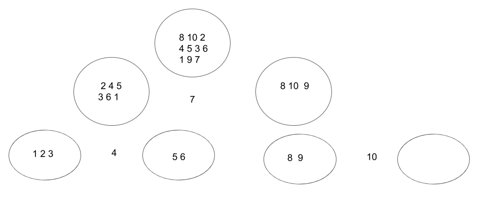
Shell sort performs repeated insertion sorts on selected subarrays of the original array being sorted. It involves multiple passes with changing subarrays. Figure 1 shows the operation of shell sort. First it sorts the subarrays containing values that have a gap between them of 5. Then it sorts the subarrays containing values with a gap of 2, and then it sorts the values that are beside each other (a gap of 1). The sort technique used on each subarray is insertion sort and the values in the subarrays are shown in blue. For example, when \(gap=2\), the algorithm sorts the subarrays [3, 1, 5, 10, 9] and [6, 4, 8, 2, 7]. Each subarray is sorted using insertion sort. The gaps in this example have been arbitrarily chosen. The code we provide in the Sorting lab uses a gap value based upon the size of the array being sorted, which is a simpler, less arbitrary approach, but not necessarily an improvement on the algorithm. How gaps are chosen is discussed in Shellsort.
n: values to be compared
n: values moved
| 8 | 10 | 2 | 4 | 5 | 3 | 6 | 1 | 9 | 7 |
| gap = 4 | |||||||||
|---|---|---|---|---|---|---|---|---|---|
| 8 | 10 | 2 | 4 | 5 | 3 | 6 | 1 | 9 | 7 |
| 5 | 10 | 2 | 4 | 8 | 3 | 6 | 1 | 9 | 7 |
| 5 | 10 | 2 | 4 | 8 | 3 | 6 | 1 | 9 | 7 |
| 5 | 3 | 2 | 4 | 8 | 10 | 6 | 1 | 9 | 7 |
| 5 | 3 | 2 | 4 | 8 | 10 | 6 | 1 | 9 | 7 |
| 5 | 3 | 2 | 4 | 8 | 10 | 6 | 1 | 9 | 7 |
| 5 | 3 | 2 | 4 | 8 | 10 | 6 | 1 | 9 | 7 |
| 5 | 3 | 2 | 1 | 8 | 10 | 6 | 4 | 9 | 7 |
| 5 | 3 | 2 | 1 | 8 | 10 | 6 | 4 | 9 | 7 |
| 5 | 3 | 2 | 1 | 8 | 10 | 6 | 4 | 9 | 7 |
| 5 | 3 | 2 | 1 | 8 | 10 | 6 | 4 | 9 | 7 |
| 5 | 3 | 2 | 1 | 8 | 7 | 6 | 4 | 9 | 10 |
| gap = 1 | |||||||||
| 5 | 3 | 2 | 1 | 8 | 7 | 6 | 4 | 9 | 10 |
| 3 | 5 | 2 | 1 | 8 | 7 | 6 | 4 | 9 | 10 |
| 3 | 5 | 2 | 1 | 8 | 7 | 6 | 4 | 9 | 10 |
| 2 | 3 | 5 | 1 | 8 | 7 | 6 | 4 | 9 | 10 |
| 2 | 3 | 5 | 1 | 8 | 7 | 6 | 4 | 9 | 10 |
| 1 | 2 | 3 | 5 | 8 | 7 | 6 | 4 | 9 | 10 |
| 1 | 2 | 3 | 5 | 8 | 7 | 6 | 4 | 9 | 10 |
| 1 | 2 | 3 | 5 | 8 | 7 | 6 | 4 | 9 | 10 |
| 1 | 2 | 3 | 5 | 8 | 7 | 6 | 4 | 9 | 10 |
| 1 | 2 | 3 | 5 | 7 | 8 | 6 | 4 | 9 | 10 |
| 1 | 2 | 3 | 5 | 7 | 8 | 6 | 4 | 9 | 10 |
| 1 | 2 | 3 | 5 | 6 | 7 | 8 | 4 | 9 | 10 |
| 1 | 2 | 3 | 5 | 6 | 7 | 8 | 4 | 9 | 10 |
| 1 | 2 | 3 | 4 | 5 | 6 | 7 | 8 | 9 | 10 |
| 1 | 2 | 3 | 4 | 5 | 6 | 7 | 8 | 9 | 10 |
| 1 | 2 | 3 | 4 | 5 | 6 | 7 | 8 | 9 | 10 |
| 1 | 2 | 3 | 4 | 5 | 6 | 7 | 8 | 9 | 10 |
| 1 | 2 | 3 | 4 | 5 | 6 | 7 | 8 | 9 | 10 |
Shell sort uses a sequence \(h_1, h_2, \ldots, h_t\) called the gap sequence such that \(h_t>h_{t-1}>\ldots>h_2>h_1\). Any increment sequence will be okay as long as \(h_1 = 1\). Here is the algorithm:
for \(h\) in (\(h_t,\ldots,h_2,h_1\))
Sort all
subarrays with values that are \(h\) apart with an insertion sort
Therefore, all values spaced \(h\) apart are sorted after each iteration. In other words, \(a[i] ≤ a[i+h]\) for all \(i\).
The last step of the algorithm sorts the value that are one apart (\(h=1\)). Therefore, the last step is a simple insertion sort. However, the previous steps help eliminate turtles (small values near the end of the array), which make insertion sort particularly inefficient, since it takes a great number of shift to move a small value from the right end of the array to the left end. Therefore, the insertion sort in the last step becomes very efficient since the big moves are done. Remember, if the input array is sorted, insertion sort is very efficient and takes \(O(n)\) to run.
Array-Based Shell Sort Implementation
Code Listing 1 shows the implementation of shell sort. Looking at the code you see it is very similar to insertion sort. It repeatedly runs insertion sorts on subarrays that are \(h\) apart while \(h\) varies from \(n/2\) to 1. The gap is decreased each loop through the list until it is 1.
There are different sequences that could be used. The sequence used in \(n/2, \ldots, h_i, \ldots, h_1\) where \(h_i=h_i+1 / 2\) and \(h_1=1\). This sequence is called Shell's increment. The shrink factor, the amount by which the gap values is divided to get a new gap value, has a strong effect on the efficiency of the sort. Empirical experimentation has shown that a ratio between gap numbers of approximately 2.2 is the best.
    def shell_sort(a):
        n = len(a)
        gap = int(n // 2.2)

        while gap > 0:

            for i in range(gap, n):
                key = a[i]
                j = i

                while j >= gap and a[j - gap] > key:
                    # Perform an insertion sort on the subarray
                    # insert a[i] in the the subarray containing
                    # values that are gap apart and before
                    # index i. The subarray is sorted.
                    a[j] = a[j - gap]
                    j = j - gap

                # put key (a[i]) in its correct place
                a[j] = key
            gap = int(gap // 2.2)
        return
Linked Shell Sort
The linked shell sort is not well suited to a linked implementation. Because arrays provide direct access to each value through an index, using a gap between indexes is trivial. Attempting to use a gap between nodes in a linked list means counting nodes across the gap until the next desired node is found. We will not implement this sort for a linked list.
Shell Sort Analysis
Although shell sort is simple to code, the runtime analysis is complex. The runtime of shell sort depends on the choice of increment sequence, but is generally \(O(n^2)\). For a detailed discussion, see: Shellsort.
The Merge Sort
This algorithm uses the divide and conquer approach which is an important algorithmic technique in Computer Science. This algorithm splits an array up into two smaller arrays, recursively sorts the two smaller arrays, and finally merges the smaller arrays back into the big array. Merge sort is a stable sort.
Merge Sort Algorithm
The merge sort algorithm works as follows. If \(n=1\), there is only one element to sort, and we are done. Otherwise it divides the array into two halves, and recursively applies merge sort on the first half and on the second half. This gives two sorted halves, which can then be merged together.
The main operation in this algorithm is merging the two sorted arrays. The following figure shows the process of merging two sorted arrays. The merging algorithm takes two sorted input arrays and one output array. It traverses the input arrays, copying the smaller of the two into the output array in each iteration. When either input array is copied completely to the output, the remainder of the other array is copied to the output array.
![The figure shows two input arrays that are merged together into an output array.
Each row shows the changes in input arrays and the output array. The first row shows
the first input array which is: [2, 4, 5, 8, 10]; the second input array which is:
[1, 3, 6, 7, 9], and the output array which is empty. One arrow is pointing to position
zero in the first input array; another arrow is pointing to the first position in the
second input array; and another arrow is pointing to first position in the output array.
In the second row, the arrow in the first array is pointing to position zero; the arrow
in the second input array is pointing to position 1; and the arrow in the output array
is pointing to position 1 which contains number one now. In the third row, the arrow in
the first array is pointing to position two; the arrow in the second input array is pointing
to position 1; and the arrow in the output array is pointing to position 2 which contains
number two now. In the fourth row, the arrow in the first array is pointing to position two;
the arrow in the second input array is pointing to position three; and the arrow in the
output array is pointing to position 3 which contains number three now. In the fifth row,
the arrow in the first array is pointing to position three; the arrow in the second input
array is pointing to position three; and the arrow in the output array is pointing to position
4 which contains number 4 now. In the sixth row, the arrow in the first array is pointing to
position four; the arrow in the second input array is pointing to position three; and the arrow
in the output array is pointing to position 5 which contains number 5 now. In the seventh row,
the arrow in the first array is pointing to position four; the arrow in the second input array
is pointing to position four; and the arrow in the output array is pointing to position 6 which
contains number 6 now. In the eight row, the arrow in the first array is pointing to position
four; the arrow in the second input array is pointing to position five; and the arrow in the
output array is pointing to position 7 which contains number 7 now. In the ninth row, the arrow
in the first array is pointing to position five; the arrow in the second input array is pointing
to position five; and the arrow in the output array is pointing to position 8 which contains
number 8 now. In the tenth row, the arrow in the first array is pointing to position five; the
arrow in the second input array is pointing to one after the last position; and the arrow in the
output array is pointing to position 9 which contains number 9 now. In the last row, the arrow
in the first array is pointing to one after the last position; the arrow in the second input array
is pointing to one after the last position; and the arrow in the output array is pointing to
position 10 which contains number 10 now.](../images/L12_F07.png)
Created by Masoomeh Rudafshani. Used with permission.
The time to merge two sorted arrays is linear, where \(n\) is the total number of elements. The reason is that at most \(n-1\) comparisons are made, and every comparison adds at least an element to the output. The last comparison may add two or more, depending on the number of remaining elements in the other array. The \(O(n)\) runtime is possible because the arrays are sorted and an extra array is used.
![The figure shows the array [68, 89, 45, 10, 20] is divided into two subarrays:
[68, 89, 45] and [10, 20]. Then the array [68, 89, 45] is divided into two subarrays [68, 89] and [45].
The array [10, 20] is divided into two subarrays [10] and [20]. The array [68, 89] is divided into two
subarrays [68] and [89]. The arrays [10] and [20] are merged together to form the array [10, 20]. The
arrays [68] and [89] are merged to form array [68, 89]. The array [68, 89] and [45] are merged together
to form array [45, 68, 89]. The arrays [45, 68, 89] and [10, 20] are merged together to form the sorted
array [10, 20, 45, 68, 89].](../images/L12_F08.png)
Created by Masoomeh Rudafshani. Used with permission.
Array-Based Merge Sort Implementation
Note the use of a an auxiliary function in this implementation of the merge sort, so that its function signature matches those of the other sorts we've seen, i.e the only parameter at the top level is the list to be sorted.
    def merge_sort(a):
        _merge_sort_aux(a, 0, len(a) - 1)
        return

    def _merge_sort_aux(a, first, last):
        if first < last:
            middle = (last - first) // 2 + first
            _merge_sort_aux(a, first, middle)
            _merge_sort_aux(a, middle + 1, last)
            _merge(a, first, middle, last)
        return

    def _merge(a, first, middle, last):
        temp = []
        i = first
        j = middle + 1

        while i <= middle and j <= last:

            if a[i] <= a[j]:
                # put leftmost element of left array into temp array
                temp.append(a[i])
                i += 1
            else:
                # put leftmost element of right array into temp array
                temp.append(a[j])
                j += 1

        # copy any remaining elements from the left half
        while i <= middle:
            temp.append(a[i])
            i += 1

        # copy any remaining elements from the right half
        while j <= last:
            temp.append(a[j])
            j += 1

        # copy the temporary array back to the passed array
        for i in range(len(temp)):
            a[first + i] = temp[i]
        return
Linked Merge Sort
The linked merge sort, like the other linked sorts we've seen, moves nodes, not data. Because of this we don't need the extra storage of a temporary array. (We do need extra temporary List headers, but they are trivial in size.) Note that unlike the array-based algorithm, this version requires an explicit splitting function, as we cannot simply use indexes to split the list. This algorithm splits a list by count, but could also move the nodes alternate from the source list to the left and right lists, amongst other possible approaches.
    def merge_sort(a):
        if a._count >= 2:
            # Split the list only if there are at least two elements.
            # Generate the left and right lists.
            left, right = Sorts._merge_split(a)
            # Sort the left list.
            merge_sort(left)
            # Sort the right list.
            merge_sort(right)
            # Merge the left and right lists back into a.
            _merge(a, left, right)
        return

    def _merge_split(source):
        # Split the list by count.
        count = source._count // 2
        curr = source._front

        for _ in range(count - 1):
            curr = curr._next

        # Define the left list.
        left = List()
        left._front = source._front
        left._rear = curr
        left._count = count
        # Define the right list.
        right = List()
        right._front = curr._next
        right._rear = source._rear
        right._count = source._count - count
        # Break the link between the two lists.
        left._rear._next = None
        # Empty the source list.
        source.clear()
        return left, right

    def _merge(target, left, right):
        # Traverse left and right appending larger value to rear of target.
        while left._front is not None and right._front is not None:

            if left._front._value <= right._front._value:
                target._move_front_to_rear(left)
            else:
                target._move_front_to_rear(right)

        # Append the remaining list - O(1) operation.
        if left._front is not None:
            target._append_list(left)
        elif right._front is not None:
            target._append_list(right)
        return
Merge Sort Analysis
First let's analyze the merge step. The merge step can be done in-place (i.e. working only with the current array), or by using a temporary array to hold the values while being merged. Using a temporary array leads to a simpler algorithm, and makes the merging to run in \(O(n)\) as discussed earlier, but requires extra storage space. If the merge step is done without an extra array, then it takes \(O(n^2)\) to merge two sorted arrays. For linked lists, however, there is no need for a temporary array as nodes can be merged back together quite easily. Therefore, the merge step would be \(O(n)\) using linked-lists.
Since merge sort is a recursive algorithm, assuming the merge step takes \(O(n)\), we can form a recurrence relation:
\(T(n) = 2 T(n/2) + O(n)\)
This relation is valid for both average case and worst case. Also, \(T(0)=T(1)=1\). It is a standard recurrence relation and the answer is \(O(n\log n)\).
If the merge step takes \(O(n^2)\), the recurrence relation would turn to
\(T(n) = 2T(n/2) + n^2\)
which result is a \(O(n^2)\) merge sort.
Merge sort is one of those algorithms that is easier to understand if implemented recursively.
The Quick Sort
Like the merge sort, this algorithm uses the divide and conquer approach. This algorithm splits an array up into two smaller arrays, recursively sorts the two smaller arrays, and finally merges the smaller arrays back into the big array. Quick sort is a stable sort.
Quick Sort Algorithm
The basic idea is that one value is picked as the pivot. Then, the values are partitioned into two sets, one containing values less than the pivot and one containing the values larger than the pivot. Then the two smaller set are sorted recursively using the same algorithm:
Created by Masoomeh Rudafshani. Used with permission.
The quick sort algorithm
- If the number of values in an array is zero or one, then return
- Pick one value as pivot
- We can choose any value, such as the first, last, middle or some other arbitrary value; however, some choices are better. For example, if we choose the first value in a sorted array, then one set will be always empty and the number of values in the other set decreases linearly. So, the algorithm takes more time. In our array-based solution we pick the middle value in the array as the pivot value. In a linked solution we always pick the front because moving to the middle of the list is non-trivial.
- Partition the array into two (possibly empty) subarrays. Our goal here is to move all values less than the pivot to the left subarray and all values larger than the pivot to the right subarray, and the pivot in between.
There are different strategies to partition the values. The one described here is easy to understand and implement.
- The first step is to swap the pivot with the last value.
- Then we initialize two indices \(i\) and \(j\), where \(i\) points to the beginning of the array and \(j\) points to the second to the last value.
- We move i to the right until we see an value larger than the pivot (\(i\) does not move if it is already pointing to an value larger than pivot). Similarly, we move \(j\) to the left until we see an value smaller than the pivot (\(j\) does not move if it is already pointing to an value smaller than pivot). When we stop, we swap the array values at positions \(i\) and \(j\) if \(i\) is to the left of \(j\) and then repeat this step by moving \(i\) and \(j\). if \(j\) is to the left of \(i\), this step is done.
- At the end, swap \(a[i]\) with the pivot (last value). Once positioned, pivot values never move.
- Recursively sort the left and right subarrays obtained by partitioning.
The partitioning process is shown in Figure 2 and the operation of quick sort is shown in Figure 3.
![The figure shows two examples of partitioning in quick sort. On the left,
there is this array: [68, 89, 54, 10, 20] that is going to be partitioned. First
45 is picked as pivot and circled around. Then 45 is swapped with 20 which is the
last value. The, index i is initialized to point to 68 and index j is initialized
to points to 10. i is moved to the right and j is moved to the left. i stops at 89
and j stops at 20 and then 89 and 20 are swapped. Then i moves to point to 89 at its
new position and j moves to point to 20 at its new position. The movement stops and
there is no swap. the pivot (last value) is swapped with the value pointed to by
i (89). On the right, there is this array: [10, 20] that is being partitioned. First
10 is picked as pivot and circled around. Then 10 is swapped with 20 which is the last
value. Then, index i is initialized to point to 20 and index j is initialized to
point to 20. i stays at its place but j is moved to the left. No swap is done since
i > j. At the end pivot and the value in position i are swapped. In other words,
10 and 20 are swapped. 10 is placed in its correct position and it is turned red. Now
the array containing 20 should be sorted which is sorted already since contains just
one value.](../images/L12_F10.png)
The left side shows the partitioning of the array: [68, 89, 45, 10, 20]. The right side shows the partition of the subarray [10, 20] obtained after initial partition (shown on the left).
Created by Masoomeh Rudafshani. Used with permission.
![The figure shows the process of quick sort on the array [68, 89, 45, 10, 20].
First 45 is picked as pivot and the array is divided into [10, 20] and [68, 89] and
position of 45 is fixed. Then subarray [10,20] is divided into two, and 10 is picked
as the pivot, and the subarray is divided into [] and [20] and the position of 10 is
fixed. [] and [20] are sorted and therefore the position of 20 is fixed as well. In
the subarray [68, 89], 68 is picked as pivot and the subarray is divided into [] and [89]
and the positions of 68 as pivot and 89 as the only value in the subarray are fixed.](../images/L12_F11.png)
The operation of quick sort algorithm on the array [68, 89, 45, 10, 20]. First 45 is picked as pivot and the array is divided into [10, 20] and [68, 89] and position of 45 is fixed (is shown in red). The process is repeated for each subarray.
Created by Masoomeh Rudafshani. Used with permission.
Array-Based Quick Sort Implementation
Note the use of a an auxiliary function in this implementation of the quick sort, so that its function signature matches those of the other sorts we've seen, i.e the only parameter at the top level is the list to be sorted.
The auxiliary function initializes \(i\) to the beginning and \(j\) to 1 past the last position in the array. We need the extra check (while \(i≤j\)) in both lines to make sure \(j\) does not go past the beginning of array and \(i\) does not go past the end of the array (going past either end by 1 is OK).
    def quick_sort(a):
        _quick_sort_aux(a, 0, len(a) - 1)
        return

    def _quick_sort_aux(a, first, last):
        # Sort the subarray a[first:last] of array a into ascending order.
        if first < last:
            p = _partition(a, first, last)
            _quick_sort_aux(a, first, p - 1)
            _quick_sort_aux(a, p + 1, last)
        return

    def _partition(a, first, last):
        # Partitions a[first:last] into a[first:pivot] and a[pivot+1:last].
        pivot = (first + last) // 2
        low = first
        high = last - 1  # After we remove pivot it will be one smaller
        pivot_value = a[pivot]
        a[pivot] = a[last]

        while low <= high:
            while low <= high and a[low] < pivot_value:
                low = low + 1
            while low <= high and a[high] >= pivot_value:
                high = high - 1
            if low <= high:
                a[low] = a[high]
        a[last] = a[low]
        a[low] = pivot_value
        # Return the new pivot position.
        return low
Linked Quick Sort
The linked quick sort, like the other linked sorts we've seen, moves
nodes, not data. We need extra temporary List headers, but they are
trivial in size. This algorithm splits a list by pivot value, which is
taken from the front of the list to split, as that is the simplest value
to access. (Moving to the middle of the list is non-trivial.) Three
separate lists are created so that once we find values equal to the
pivot value we don't have to deal with them again. The _append_list
helper method reconnects the Lists with an efficiency of \(O(1)\) since
it doesn't have to move data between Lists one at a time.
    def quick_sort(a):
        if a._front is not None:
            # Partition the list into three with respect to pivot value.
            lesser, equals, greater = _partition(a)
            quick_sort(lesser)
            quick_sort(greater)
            # Put all three lists back together in order.
            if lesser._front is not None:
                a._append_list(lesser)
            # equals list contains at least the pivot value.
            a._append_list(equals)
            if greater._front is not None:
                a._append_list(greater)
        return

    def _partition(source):
        lesser = List()
        greater = List()
        equals = List()
        # Move source front node to the equals list.
        equals._move_front_to_rear(source)
        pivot = equals._front

        while source._front is not None:
            # Process the remaining nodes with respect to the pivot node.
            if pivot._value > source._front._value:
                lesser._move_front_to_rear(source)
            elif pivot._value < source._front._value:
                greater._move_front_to_rear(source)
            else:
                equals._move_front_to_rear(source)
        return lesser, equals, greater
Quick Sort Analysis
The quick sort is a recursive algorithm, and we need to find the recurrence formula. The running time of quick sort is equal to the running time of the two recursive calls plus the linear time spent in the partition (pivot is picked randomly and its selection takes constant time). Therefore, the recurrence relation would be:
\(T(n)=T(i)+T(n-i-1)+cn\)
where \(i\) is the number of values in the first partition. Also, \(T(0)=T(1)=1\).
In the worst-case (e.g., where pivot is the smallest value all the time), one partition does not contain any value and the other partition contains the rest of the values, and the recurrence relation turns to
\(T(n)=T(0)+T(n-1)+cn\).
which means \(T(n)=O(n^2)\).
In the best case, each time the pivot is in the middle. Two partitions are half of the size of the original and therefore, \(T(n)=2T(n/2)+cn\) which means \(T(n)=O(n\log{n})\).
The average case is also shown to be \(O(n\log{n})\). We skip the mathematical analysis here but the idea is to find the average value of \(T(i)\) and \(T(n-i-1)\). Refer to Quicksort for a complete analysis.
Non-Comparison Sorts
The earlier sorting methods discussed are all comparison based sorts, and the best time complexity we can expect from them is \(O(n\log{n})\). However, there are non-comparison based sorts that run in linear time, \(O(n)\). We will look in particular at the counting sort and the radix sort.
The Counting Sort
The main idea is to sort the values of an array into buckets, and for the buckets to contain the counts of the values, not the values themselves. The values act as indexes to the buckets. For this sort to work you must know the range of values in the array to sort. Then you need to assign one bucket for each value in the range. For example, if the array contains integers from 1 to 99 you must have 99 buckets indexed with 1 to 99. Each bucket contains a running count. The you walk through the input array, and for the value \(i\) in the array, you increment the count in bucket \(i\) by 1. After reading the entire input array, use the counts to reconstruct the sorted array. This is not a stable sort.
The Array-Based Counting Sort Implementation
    def counting_sort(a):
        if len(a) > 0:
            # Find the largest value in a and set up a counting
            # array with a size of the value range.
            counting = [0] * (max(a) + 1)

            # Store the count for each value.
            for v in a:
                counting[v] += 1

            i = 0

            for v in range(len(counting)):
                for _ in range(counting[v]):
                    # Copy each value counting[v] times back into a.
                    a[i] = v
                    i += 1
            return
The Linked Counting Sort Implementation
This is not a useful sort for a linked structure, as it would require deleting and creating List nodes according to a count instead of just temporarily moving the nodes. A better linked approach would be a bucket sort in which, like the counting sort, an array of buckets is created, but each bucket is a List, and nodes are moved to one of these Lists by using their value as an index. Once the original list is exhausted, all nodes would be moved back to the original List bucket by bucket. Implementing this sort is left as an exercise to you.
The Counting Sort Analysis
The runtime is \(O(n+k)\) where \(n\) is the number of values in input array and \(k\) is the range of input. If \(n==k\) as is often the case, the runtime would be \(O(n)\) (linear) time. The extra space is \(O(k)\), where an array of size \(k\) is used (each cell is a bucket) is used to store the counts.
The Radix Sort
Counting sort is a linear time sorting algorithm that sorts in O(n+k) time when elements are in the range from 1 to k. However, if the elements are in the range from 1 to \(n^2\) then the counting sort takes \(O(n^2)\) which is worse than comparison-based sorting algorithms. To sort such an array in linear time we can use radix sort.
Radix Sort Algorithm
The radix algorithm sort numbers based on their digits (i.e. by radix): it starts sorting from least significant digit to most significant digit. It applies to sorting \(n\) numbers in the range 0 to \(n^p-1\) for some \(p\). It consists of successive bucket-style sorts. In the base 10 version (there are others), imagine that there are 10 buckets labeled 0 to 9. Into any bucket \(i\) goes all numbers whose 1s digit is \(i\). Then concatenate the contents of the buckets in order and sort again. This time bucket \(i\) gets all numbers whose 10s digit is \(i\). You may keep making passes with the 100s digit, the 1000s digit, etc.
Since the number of passes to make through the array of values to process is based upon the radix of the largest number in that array, you must find the largest number in the array and determine how many digits it contains. This should be done with a \(\log_{10}\) calculation - this is left as an exercise for you.
Assume we have the following list: [99, 82, 53, 78, 18, 72]
The radix sort on this list looks like:
a |
[99, 82, 53, 8, 18, 72] |
buckets1s Column |
[[], [], [82, 72], [53], [], [], [], [], [8, 18], [99]] |
a |
[82, 72, 53, 8, 18, 99] |
buckets10s Column |
[[8], [18], [], [], [], [53], [], [72], [82], [99]] |
a |
[8, 18, 53, 72, 82, 99] |
In more detail: the algorithm considers each number by its current radix,
or digit. On the first pass, each number is first placed into a bucket
indexed according to the value in its 1 radix, i.e by it's one digit. On
the second pass, each number is placed into a bucket indexed according
to its 10s digit. (Where a digit does not exist, as in the number 8,
it is treated as 0.) If there were 100s digits, there would
be a third pass with the bucket chosen for its 100s digit. The number of
passes is equal to the number of digits in the largest number in the
list to be sorted. (In this particular algorithm values are popped from
the ends of the lists.) Sorting the list above then becomes:
| 10's | 1's |
| 1 | 5 |
| 2 | 3 |
| 4 | 5 |
| 1 | 2 |
| 7 | 8 |
| 6 | 1 |
| 7 | |
| 1 | 8 |
| 2 | 4 |
| Index | Values |
| 0 | [] |
| 1 | [61] |
| 2 | [12] |
| 3 | [23] |
| 4 | [24] |
| 5 | [45, 15] |
| 6 | [] |
| 7 | [7] |
| 8 | [18, 78] |
| 9 | [] |
| 10's | 1's |
| 6 | 1 |
| 1 | 2 |
| 2 | 3 |
| 2 | 4 |
| 1 | 5 |
| 4 | 5 |
| 7 | |
| 7 | 8 |
| 1 | 8 |
| Index | Values |
| 0 | [7] |
| 1 | [18, 15, 12] |
| 2 | [24, 23] |
| 3 | [] |
| 4 | [45] |
| 5 | [] |
| 6 | [61] |
| 7 | [78] |
| 8 | [] |
| 9 | [] |
Final a:
[7, 12, 15, 18, 23, 24, 45, 61, 78]
Radix Sort Implementation
The radix sort can be implemented for both array-based and linked data structures. It can work with data that has a well-defined radix, i.e. data like integers or strings that allow you to pick off individual digits or characters. Implementing it for complex data such as Food or Movie classes without identifiable radixes is problematic, if even possible. Implementing this sort may be left as an exercise to you.
Radix Sort Analysis
The runtime of radix sort is \(θ(d(n + k))\) where \(d\) is the maximum number of digits in numbers, \(k\) is the number of possible values for a digit, and a linear-time algorithm like counting sort is used. When \(d\) is constant and \(k= O(n)\), the radix sort time efficiency is \(O(n)\) (linear).
Summary
In this lesson, we introduced several sorting algorithms with different runtimes. We studied a number of comparison-based algorithms such as bubble sort, insertion sort which have \(O(n^2)\) runtime in worst case and average case. We also studied a number of other algorithms which run in \(O(n\log{n})\) in worst case and average case. We studied merge sort which is \(O(n\log{n})\) in worst case and average case and it is easy to develop the code, but it requires \(O(n)\) extra space. We also studied quick sort which is \(O(n^2)\) in the worst case, and \(O(n\log{n})\) in average case. Although the runtime gives us a good idea of how fast an algorithm is, in practice the choice of an algorithm depends on the input size. For example, for small input size insertion sort runs faster.
Swapping is the fundamental operation in many sorting algorithms. In our discussion on sorting algorithms, we assumed that the data elements are integers, and so swapping is not expensive. In practice, we usually need to sort complex objects by a certain key. For example, we may need so sort an array of student objects by student id. The objects could be large and contain many attributes and methods which make swapping very expensive. However, if the input array contains pointer to an object, then swapping the pointers is not much different from swapping the integer numbers.
We also introduced a number of sorting algorithms such as counting sort and radix sort that run in linear time. The \(O(n)\) runtime is possible because these algorithms have some assumptions about the input array.
That concludes our discussion of the topics covered in this course. We discussed some of the important ADTs and data structures in Computer Science such as List, Stack, Queue, and Priority Queue ADTs as well as data structures such as arrays, linked-lists, binary search trees, heap data structures, and hash tables. We also discussed few algorithm development techniques throughout the course such as searching, recursion, divide-and-conquer, and backtracking. We also discussed how to estimate the runtime of an algorithm. In later course, you get to implement the ideas taught here in other programming languages. In addition, you will learn about more algorithmic techniques and more advanced data structures.
The topics you have learned in this course are important in all other parts of the Computer Science, and if you continue in this field, you will use to the topics discussed here in your future courses and your future jobs.
References
- Data Structures and Algorithm Analysis in C++, Mark Allen Weiss. 2006.
- CSE373: Data Structures and Algorithms, School of Computer Science and Engineering at University of Washington, Notes on Sorting
- Introduction to Algorithms, Thomas H. Cormen, Charles E. Leiserson, Ronald L. Rivest, Clifford Stein. The MIT Press, 2001.
- Sorting, Wikipedia